Discrete Event Simulation Engineering
Copyright © 2021-2024 Gerd Wagner
Draft version, published 2024-02-29.

Abstract
This book explains how to design discrete event simulations with the help of the Unified Modeling Language (UML) and the Discrete Event Process Modeling Notation (DPMN) and how to implement DPMN models with the JavaScript simulation framework OESjs as well as with the Discrete Event Simulation tools Simio and AnyLogic. DPMN is based on the Object Event Modeling and Simulation paradigm, representing a general Discrete Event Simulation approach based on Object-Oriented Modeling and Event Scheduling.
Essentially, DPMN has been developed by incrementally extending Event Graphs by adding increasingly high-level modeling concepts. In the first step, we add the concept of objects, resulting in Object Event Graphs. In the second step, we add the concept of (resource-constrained) activities, resulting in the Activity Network modeling language DPMN-AN. In the third step, we add the concept of processing activities, resulting in the Processing Network modeling language DPMN-PN.
This book has a companion: Business Process Modeling and Simulation with DPMN, with which it has a large overlap.
This book is available in the following versions: Open Access HTML ebook PDF Restricted Access HTML
Table of Contents
- List of Figures
- List of Tables
- I. Introduction
- II. Event-Based Simulation
- III. Activity-Based Simulation and Activity Networks
- 8. Simple Activities
- 9. Resource-Constrained Activities
- 10. Case Studies
- IV. Processing Activities and Processing Networks
- V. Agent-Based Modeling and Simulation
- Appendices
- Bibliography
- Index
List of Figures
- 1-1. From conceptualization via design to implementation
- 2-1. The entity types Shop and Delivery.
- 2-2. Adding properties and operations.
- 2-3. Adding a property constraint and an operation constraint.
- 2-4. Object and event types as two different categories of entity types.
- 2-5. A BPMN Process Diagram for a pizza service company
- 2-6. A DPMN Process Diagram for a pizza service company
- 3-1. A basic DPMN Process Diagram showing an Object Event Graph.
- 3-2. A basic OE class model defining an object type and three event types.
- 3-3. A DPMN-A process model and its underlying OE class model
- 3-4. A DPMN-A process model with an RDAS arrow and its underlying OE class model
- 3-5. A DPMN-A process model of a Load-Haul-Dump business process
- 3-6. A process design for the Make-and-Deliver-Pizza business process.
- 3-7. An enriched process design model
- 3-8. An OE class design model for the Make-and-Deliver-Pizza business process.
- 5-1. A basic DPMN Process Diagram showing an OEG.
- 5-2. A basic OE class model defining an object type and three event types.
- 7-1. A conceptual information model of a manufacturing workstation system
- 7-2. A conceptual process model of a manufacturing workstation system
- 7-3. An information design model
- 7-4. A process design model in the form of a DPMN Process Diagram
- An example of a simple AN
- 8-1. Introducing an activity type in a conceptual information model of a single workstation system.
- 8-2. Introducing an activity type in a conceptual process model of a single workstation system.
- 8-3. Going from basic OEM to OE class models by introducing activity types.
- 8-4. Going from basic DPMN to DPMN-A process models by introducing Activity rectangles.
- 8-5. Allocating the workstation as a resource of Processing activities
- 9-1. Typically, the performer of an activity is a resource object.
- 9-2. Activity types may have special properties representing resource roles.
- 9-3. A conceptual information model of the activity type "examinations" with resource roles.
- 9-4. A conceptual process model based on the information model of Figure 9-3.
- 9-5. A conceptual information model with doctors and patients as people.
- 9-6. Adding the activity type "walks to room" to the conceptual information model.
- 9-7. A conceptual process model based on the information model of Figure 9-6.
- 9-8. An improved process model based on the information model of Figure 9-6.
- 9-9. Displaying the process owner and activity performers in a conceptual process model.
- 9-10. Adding parallel participation multiplicities for rooms participating both in walks and examinations at the same time.
- 9-11. An information model for the simplified design with the resource counters nmrOfRooms and nmrOfDoctors.
- 9-12. A process design model based on the information design model of Figure 9-11.
- 9-13. An OE class model with resource object types for modeling resource roles and pools.
- 9-14. A process design model based on the information design model of Figure 9-13.
- 9-15. Any resource type
R extends the pre-defined object type
Resource - 9-16. A simplified version of the model of Figure 9-13
- 9-17. An OE Class Diagram modeling a single workstation system with resource-constrained processing activities
- 9-18. An information design model for decoupling the allocation of rooms and doctors.
- 9-19. A process design model based on the information design model of Figure 9-18.
- 9-20. Representing the process owner as a Pool and activity performers as Lanes in a process design model.
- 9-21. A conceptual modeling pattern for a sequence of resource-constrained activities
- 9-22. Using RDAS arrows in a conceptual process model.
- 9-23. Displaying the implicit allocate-release steps.
- 9-24. Modeling WorkStation as a resource type
- 9-25. A simplified version of the workstation process model using an RDAS arrow.
- 9-26. A simplified version of the medical department information model with Doctor and Room as resource types
- 9-27. A simplified version of the medical department process model using RDAS arrows.
- 9-28. Doctors perform examinations.
- 9-29. An examination requires two resources: a room and a doctor.
- 9-30. The class Examination implementing the corresponding activity type.
- 9-31. The loading of a truck requires at least one, and can be handled by at most two, wheel loaders.
- 9-32. The class LoadTruck implementing the corresponding activity type.
- 9-33. An examination room may be used by up to 3 examinations at the same time.
- 9-34. The teaching of a course is performed by teachers.
- 10-1. An information design model defining object, event and activity types.
- 10-2. A process design for the Make-and-Deliver-Pizza business process
- 10-3. An enriched process design model
- 10-4. A DPMN process design model for the Make-and-Deliver-Pizza business process.
- 10-5. An AnyLogic process diagram for the Make-and-Deliver-Pizza business process.
- 10-6. A DPMN process design model for the Make-and-Deliver-Pizza business process.
- 10-7. A Simio process diagram for the Make-and-Deliver-Pizza business process.
- 10-8. A conceptual OE class model describing object, event and activity types.
- 10-9. A refined conceptual process model.
- 10-10. An information design model for the Load-Haul-Dump system.
- 10-11. A computationally complete process design for the Load-Haul-Dump business process.
- 10-12. A
design model for the
HaulRequestevent rule. - 10-13. A design
model for the
GoToLoadingSiteevent rule. - 10-14. A design model for the
Loadevent rule. - 10-15. A design model for the
Haulevent rule. - 10-16. A
design model for the
Dumpevent rule. - 10-17. A design model for the
GoBackToLoadingSiteevent rule. - 10-18. An AnyLogic process diagram for the Load-Haul-Dump business process.
- 10-19. A Simio process diagram for the Load-Haul-Dump business process.
- Resource-constrained activities involving processing objects are processing activities.
- 11-1. A conceptual OEM class model defining built-in types for conceptual PN modeling
- 11-2. A PN model using the new DPMN modeling elements of PN Node rectangles, Processing Flow arrows and Object-Event Flow arrows
- 11-3. A DPMN-PN process diagram with an Event Scheduling arrow
- 12-1. An OEM class design model defining built-in types for making PN design models
- 12-2. A PN model of a workstation system using PN Node rectangles and PN Flow arrows
- 12-3. A PN model of a workstation system where parts may have to be reworked
- 12-4. A PN model using the new DPMN modeling elements of PN Node rectangles and PN Flow arrows
List of Tables
Part I. Introduction
Chapter 1. Basic Concepts
1.1. What Is Discrete Event Simulation?
The term Discrete Event Simulation (DES) has been
established as an umbrella term subsuming various kinds of computer
simulation approaches, all based on the general idea of modeling
entities/objects and events. In the DES literature, it is often stated that
DES is based on the concept of entities flowing through the system
(more precisely, through a queueing network
). This is the paradigm of
an entire class of simulation software in the tradition of GPSS (Gordon,
1961) and SIMAN/Arena (Pegden &
Davis, 1992). However, this paradigm characterizes a special (yet
important) class of DES only, it does not apply to all discrete event
systems.
Pegden (2010) explains that the 50 year history of DES has been shaped by three fundamental paradigms: Markowitz, Hausner and Karr (1962) pioneered the Event-Based Simulation paradigm with SIMSCRIPT, Gordon (1961) pioneered the Processing Network paradigm[1] with GPSS, and Dahl and Nygaard (1967) pioneered Object-Orientation and the (co-routine-based) Process Interaction paradigm with Simula.
While the concept of an event is often limited to instantaneous events in the area of DES, the general concept of an event, as discussed in philosophy and in many fields of computer science, includes composite events and events with non-zero duration.
A discrete event system (or discrete dynamic system) consists of
- objects (of various types) having a state (consisting of qualities) and dispositions, and
- events (of various types) triggering certain dispositions of objects participating in them,
such that the states of affected objects may be changed by events according to the dispositions triggered by them. It is natural to consider the concept of discrete events, occurring at times from a discrete set of time points.
For modeling a discrete event system as a state transition system, we have to describe its
- object types , e.g., in the form of classes of an object-oriented language;
- event types , e.g., in the form of classes of an object-oriented language;
- causal regularities (disposition types) e.g., in the form of event rules.
Any DES formalism has one or more language elements that allow specifying event rules representing causal regularities. These rules specify, for any event type, the state changes of objects and the follow-up events caused by the occurrence of an event of that type, thus defining the dynamics of the transition system. Unfortunately, this is often obscured by the standard definitions of DES that are repeatedly presented in simulation textbooks and tutorials.
According
to Pegden (2010), a
simulation modeling worldview provides a framework for defining
a system in sufficient detail that it can be executed to simulate the
behavior of the system
. It must precisely define the dynamic state
transitions that occur over time
. Pegden explains that the 50 year
history of DES has been shaped by three fundamental paradigms: Markowitz,
Hausner, and Karr (1962)
pioneered the event worldview with SIMSCRIPT, Gordon (1961)
pioneered the processing network worldview with GPSS, and
Dahl and Nygaard (1966)
pioneered the object worldview with Simula. Pegden
characterizes these paradigms in the following way:
Event worldview: The system is viewed as a series of instantaneous events that change the state of the system over time. The modeler defines the events in the system and models the state changes that take place when those events occur. According to Pegden, the event worldview is the most fundamental worldview since the other worldviews also use events, at least implicitly.
Processing Network worldview: The system
under investigation is described as a processing network where entities
flow through the system
(or, more precisely, work objects are routed
through the network) and are subject to a series of processing steps
performed at processing nodes through processing activities, possibly
requiring resources and inducing queues of work objects waiting for the
availability of resources (processing networks have been called queueing
networks
in Operations Research). This approach allows high-level
modeling with semi-visual languages and is therefore the most widely used
DES approach nowadays, in particular in manufacturing industries and service
industries. Simulation platforms based on this worldview may or may not
support object-oriented modeling and programming.
Object
worldview: The system is modeled by describing the objects that make
up the system. The system behavior emerges from the interaction
of
these objects.
All three worldviews lack important conceptual elements. The event worldview does not consider objects with their (categorical and dispositional) properties. The processing network worldview neither considers events nor objects. And the object worldview, while it considers objects with their categorical properties, does not consider events. None of the three worldviews includes modeling the dispositional properties of objects with a full-fledged explicit concept of event rules.
The event worldview and the object worldview can be combined in approaches that support both objects and events as first-class citizens. This seems highly desirable because (1) objects (and classes) are a must-have in today’s state-of-the-art modeling and programming, and (2) a general concept of events is fundamental in DES, as demonstrated by the classical event worldview. We use the term object-event worldview for any DES approach combining OO modeling and programming with a general concept of events.
1.2. Object Event Modeling and Simulation
Object Event (OE) Modeling and Simulation (M&S) is a new general modeling paradigm based on the two most important ontological categories: objects and events. In philosophy, objects have also been called endurants or continuants, while events have also been called perdurants or occurrents.
OEM&S combines Object-Oriented (OO) Modeling with the event scheduling paradigm of Event Graphs (Schruben 1983). The relevant object types and event types are described in an information model, which is the basis for making a process model. A modeling approach that follows the OEM paradigm is called an OEM approach. Such an approach needs to choose, or define, an information modeling language (such as Entity Relationship Diagrams or UML Class Diagrams) and a process modeling language (such as UML Activity Diagrams or BPMN Process Diagrams).
We propose an OEM approach based on Object Event (OE) Class Models (a form of UML Class Diagrams) for conceptual information modeling and information design modeling, as well as DPMN Process Diagrams for conceptual process modeling and for process design modeling.
In the proposed approach, object types and event types are modeled as special categories of classes in an OE Class Diagram. Random variables are modeled as a special category of class-level operations constrained to comply with a specific probability distribution such that they can be implemented as static methods of a class. Queues are not modeled as objects, but rather as ordered association ends, which can be implemented as collection-valued reference properties. Finally, event rules, which include event routines, are modeled in DPMN process diagrams (and possibly also in pseudo-code), such that they can be implemented in the form of special onEvent methods of event classes.
Like Petri Nets (Petri 1962) and DEVS (Zeigler 1976), OEM&S has a formal semantics. But while Petri Nets and DEVS are abstract computational formalisms without an ontological foundation, OEM&S is based on the fundamental ontological categories of objects, events and causal regularities.
In model-based simulation engineering, we distinguish between (1) a conceptual model describing a real-world problem domain, and (2) a simulation design model defining a certain computational solution for the purpose of a simulation study. Both conceptual models and design models consist of an OE class model describing/defining the system's state structure (in the form of object types and event types, and the associations between them) and a DPMN process model describing/defining the system's dynamics (in the form of causal regularities captured by event rules).
An OEM approach results in a simulation design model that can, in principle, be implemented with any object-oriented simulation technology. However, a straightforward implementation can only be expected from a technology that implements the OEM&S paradigm, such as the OES JavaScript (OESjs) framework.
The formal semantics of OEM/DPMN is based on the semantics of Event Graphs (Schruben 1983), which was originally defined in terms of integer programming. Wagner (2017a) has proposed a more general semantics of Event Graphs where such a graph is decomposed into a set of transition functions ("event rules") such that a transition system (or Abstract State Machine) semantics is obtained. This semantics can be easily extended to Object Event Graphs, as shown in Wagner (2017a). Finally, the semantics of DPMN-A models ("Activity Networks") is obtained by reduction to Object Event Graphs using two rewriting patterns, and the semantics of DPMN-PN models ("Processing Networks") is obtained by reduction to DPMN-A.
It has been an unfortunate course of the history of science that Event Graphs have not become more well-known and, instead of Event Graphs, Petri Nets have been chosen as the standard semantics of BP models, despite the fact that Event Graphs would have been a much more natural choice.
1.3. Model-Driven Engineering
Model-Driven Engineering (MDE), also called model-driven development, is a well-established paradigm in software engineering. Since simulation engineering can be viewed as a special case of software engineering, it is natural to apply the ideas of MDE also to simulation engineering.
In MDE, there is a distinction between three kinds of models as engineering artifacts created in the analysis, design and implementation phases of a development project:
- domain models (also called conceptual models), which describe a real-world domain (and are independent of a computational solution),
- design models, which define platform-independent solution designs,
- implementation models, which are platform-specific.
Domain models are solution-independent descriptions of a problem domain produced in the analysis phase. A domain model may include both descriptions of the domain's state structure (in conceptual information models) and descriptions of its processes (in conceptual process models). They are solution-independent, or computation-independent, in the sense that they are not concerned with making any system design choices or with other computational issues. Rather, they focus on the perspective and language of the subject matter experts for the domain under consideration.
In the design phase, first a platform-independent design model, as a general computational solution, is developed on the basis of the domain model. The same domain model can potentially be used to produce a number of (even radically) different design models. Then, by taking into consideration a number of implementation issues ranging from architectural styles, nonfunctional quality criteria to be maximized (e.g., performance, adaptability) and target technology platforms, one or more platform-specific implementation models are derived from the design model. These one-to-many relationships between conceptual models, design models and implementation models are illustrated in Figure 1-1.

In general, a model does not consist of just one model diagram including all viewpoints or aspects of the system to be developed. Rather it consists of a set of models, one (or more) for each viewpoint. The two most important viewpoints, crosscutting all three modeling levels (domain conceptualization, design and implementation) are
- information modeling, which is concerned with the state structure of the domain, design or implementation;
- process modeling, which is concerned with the dynamics of the domain, design or implementation.
Examples of widely used languages for information modeling are Entity Relationship (ER) Diagrams and UML Class Diagrams. Since the latter subsume the former, we prefer using UML class diagrams for making all kinds of information models, including SQL database models.
Examples of widely used languages for process modeling are (Colored) Petri Nets, UML Sequence Diagrams, UML Activity Diagrams and the BPMN. Notice that there is more agreement on the right concepts for information modeling than for process modeling, as indicated by the much larger number of different process modeling languages. This reflects a lower degree of understanding the nature of events and processes compared to understanding objects and their relationships.
Model-driven simulation engineering is based on the same kinds of models as model-driven software engineering: going from a domain model via a design model to an implementation model for the simulation platform of choice (or to several implementation models if there are several target simulation platforms). The specific concerns of simulation engineering, like, e.g., the concern to capture certain parts of the overall system dynamics with the help of random variables, do not affect the applicability of MDE principles. However, they define requirements for the modeling languages to be used.
Chapter 2. Visual Modeling
2.1. Information Modeling with UML Class Diagrams
Conceptual information modeling is mainly concerned with describing the relevant entity types of a real-world domain and the relationships between them, while information design and implementation modeling are concerned with describing the logical (or platform-independent) and platform-specific data structures (in the form of classes) for designing and implementing a software system or simulation. The most important kinds of relationships between entity types to be described in an information model are associations and subtype/supertype relationships, which are called ‘generalizations’ in UML.
In UML Class Diagrams, an entity type is described with a name, and possibly with a list of properties and operations (called methods when implemented), in the form of a class rectangle with one, two or three compartments, depending on the presence of properties and operations. Integrity constraints, which are conditions that must be satisfied by the instances of a type, can be expressed in special ways when defining properties or they can be explicitly attached to an entity type in the form of an invariant box.
An
association between two entity types is expressed as a
connection line between the two class rectangles representing the entity
types. The connection line is annotated with multiplicity expressions
at both ends. A multiplicity expression has the form
m..n where m is a non-negative natural number denoting
the minimum cardinality, and n is a positive natural number
(or the special symbol * standing for unbounded) denoting the maximum
cardinality, of the sets of associated entities. Typically, a multiplicity
expression states an integrity constraint. For instance, the multiplicity
expression 1..3 means that there are at least 1 and at most 3
associated entities. However, the special multiplicity expression
0..* (also expressed as *) means that there is no
constraint since the minimum cardinality is zero and the maximum cardinality
is unbounded.
For instance, the model shown in Figure 3 describes the entity types
Shop and Delivery, and it states that
- there are two classes:
ShopandDelivery, representing entity types; - there is a one-to-many association between the classes
ShopandDelivery, where a shop is thereceiverof a delivery.

Using further compartments in class rectangles, we can add properties and operations. For instance, in the model shown in Figure 4, we have added
- the properties name and stockQuantity to
Shopand quantity toDelivery, - the instance-level operation onEvent to
Delivery, - the class-level operation leadTime to
Delivery.

Notice that in Figure
4, each property is declared together with a datatype as its
range. Likewise, operations are declared with a (possibly empty)
list of parameters, and with an optional return value type. When an
operation (or property) declaration is underlined, this means that it is
class-level instead of instance-level. For instance, the underlined
operation declaration leadTime(): Decimal indicates that
leadTime is a class-level operation that does not take any argument
and returns a decimal number.
We may want to define various types of
integrity constraints for better capturing the semantics of entity types,
properties and operations. The model shown in Figure 5 contains an example of a property
constraint and an example of an operation constraint. These types of
constraints can be expressed within curly braces appended to a property or
operation declaration. The keyword id in the declaration of the
property name in the Shop class expresses an ID
constraint stating that the property is a standard identifier, or primary
key, attribute. The expression Exp(0.5) in the declaration of
the random variable operation leadTime in the
Delivery class denotes the constraint that the operation must
implement the exponential probability distribution function with
event rate 0.5.

UML allows defining
special categories of modeling elements called stereotypes
. For
instance, for distinguishing between object types and
event types as two different categories of entity types we can
define corresponding stereotypes of UML classes («object type» and «event
type») and use them for categorizing classes in class models, as shown in Figure 6.

Another example of using UML’s stereotype feature is the designation of an operation as a function that represents a random variable using the operation stereotype «rv» in the diagram of Figure 6.
A class may be defined as abstract by writing its name in italics, as in the example model of Figure 11. An abstract class cannot have direct instances. It can only be indirectly instantiated by objects that are direct instances of a subclass.
A good overview of the most recent version of UML (UML 2.5) is provided by www.uml-diagrams.org/uml-25-diagrams.html.
2.2. Process Modeling with BPMN and DPMN
The Business Process Modeling Notation (BPMN) is an activity-based graphical modeling language for defining business processes following the flow-chart metaphor. In 2011, the Object Management Group has released version 2.0 of BPMN with an optional execution semantics based on Petri-Net-style token flows.
The most important elements of a BPMN process model are listed in Table 2-1.
| Name of element | Meaning | Visual symbol(s) |
|---|---|---|
Event |
|
 |
Activity |
|
 |
Gateway |
A Gateway is a node for branching or merging control flows. A Gateway with an "X" symbol denotes an Exclusive OR-Split for conditional branching, if there are 2 or more output flows, or an Exclusive OR-Join, if there are 2 or more input flows. A Gateway with a plus symbol denotes an AND-Split for parallel branching, if there are 2 or more output flows, or an AND-Join, if there are 2 or more input flows. A Gateway can have both input and output flows. |
 |
Sequence Flow |
An arrow expressing the temporal order of Events, Activities, and Gateways. A Conditional Sequence Flow arrow starts with a diamond and is annotated with a condition (in brackets). |
  |
Data Object |
Data Objects may be associated with Events or Activities, providing a context for reading/writing data. A unidirectional dashed arrow denotes reading, while a bidirectional dashed arrow denotes reading/writing. |
 |
A good modeling tool, with the advantages of an online solution, is the Signavio Process Editor, which is free for academic use (www.signavio.com/bpm-academic-initiative).
BPMN process diagrams can be used for making
- conceptual process models , e.g., for documenting existing business processes and for designing new business processes;
- process automation models for specific process automation platforms (that allow partially or fully automating a business process) by adding platform-specific technical details in the form of model annotations that are not visible in the diagram.
The following diagram shows an example of a conceptual BPMN process model.

This BPMN diagram consists of a BPMN:Pool rectangle with name "pizza service" denoting the modeled business process pattern/type, which is partitioned into three BPMN:Lanes, each representing a performer (type) that participates in the process (type). Each performer type lane contains the types of activities the performers of that type are in charge of. Each type of activity may be associated with (a number of) types of objects that participate in activities of that type (often as resources).
However, the BPMN process diagram language has several semantic issues and is not expressive enough for making platform-independent process design models that can be used for designing DES models.
Shortcomings of BPMN
Notice the BPMN Boundary Timeout Event circle attached to the take order activity in Figure 2-5 representing timeout events that cancel the activity. They are supposed to model the reneging behavior of waiting customers loosing their patience and hanging up the phone without placing an order. However, BPMN does not allow restricting such a timeout mechanism to the waiting phase of a task (planned activity), that is the time span during which the task has been enqueued, but not yet started. Rather, it applies to the entire cycle time of take order activities, which means that also started activities, where the order taker is already listening to the customer, may be canceled due to reneging.
While BPMN allows modeling the performers of activities with swimlanes (referring to organizational positions with corresponding resource pools), it does not support modeling other types of resource objects, such as machines or rooms. As a workaround, the model above includes two BPMN Data Objects, ovens and scooters, for representing resource objects. Also, BPMN does not allow specifying resource multipliclity constraints (e.g., for stating that making a pizza requires two pizza makers and one oven).
The third, and most severe, issue of the BPMN model is its uniform (semantically overloaded) use of "sequence flow" arrows for sequencing both events and activities. While in the case of all three activities, incoming "sequence flow" arrows do not mean that an activity is started, but rather that a new task is enqueued (and only started when all required resources become available), in the case of the lost order event, the incoming "sequence flow" arrow means that a new event is scheduled to occur immediately.
BPMN has the following issues:
- A limited concept of "business processes" as isolated "cases", which does not allow to account for any dependency between business processes (e.g., competing for resources).
- Overloading/ambiguity of sequence flow arrows, which represent various kinds of connections, including resource-independent event flows and resource-dependent activity scheduling.
- Insufficient integration of the objects that participate in a process.
- Insufficient support of resource management. In particular, no other resources except (human) performers can be modeled, and the important concepts of resource multipliclity constraints, parallel participation constraints, resource pools, alternative resource types and task priorities are not supported.
- No support of processing activities in processing networks, which are generalized queueing networks where processing objects enter a system via arrival events at an entry station and then "flow through the system" (being subject to processing activities at processing stations) before they leave the system via departure events at an exit station.
- No convincing formal semantics. BPMN's official execution semantics is defined in terms of an abstract Petri-Net-style "token" flow (following the predominant academic paradigm), which does not match its intuitive semantics based on event flows and resource-dependent activity scheduling.
DPMN solves many issues of BPMN
The Discrete Event Process Modeling Notation (DPMN) is a Discrete Event Simulation modeling language based on Event Graphs (Schruben 1983) and BPMN. It combines the intuitive flowchart modeling style of BPMN with the rigorous semantics provided by the event scheduling arrows of Event Graphs and the event rules of the Object Event Modeling and Simulation (OEM&S) paradigm (Wagner 2017a, Wagner 2018b).DPMN adapts the language of BPMN Process Diagrams for the purpose of simulation design modeling where a process model must represent a computationally complete process specification. While large parts of BPMN’s vocabulary, visual syntax and informal semantics can be preserved in DPMN, a number of modeling elements need to be modified.
The following diagram shows the DPMN process model corresponding to the BPMN model shown in Figure 2-5 above.

DPMN adopts and adapts the syntax and semantics of BPMN in the following way:
- Instead of BPMN's "Sequence Flow" arrows, DPMN has
- Event Flow arrows, or Event Scheduling arrows, like in Event Graphs, representing the causation of follow-up events in conceptual process models, corresponding to event scheduling in process design models. For instance, in Figure 2-6, the arrow from the time out event at the "take order" task queue to the "lost orders" event is an event flow arrow.
- Resource-Dependent Activity Scheduling (RDAS) arrows with three bars representing a task queue. For instance, in Figure 2-6, "order calls" events and "take order" activities, and "take order" and "make pizza" activities, are connected via an RDAS arrow.
- A DPMN Process Diagram has an underlying UML Class Diagram defining
its types (including object, event and activity types). These type
definitions also include definitions of resource roles,
resource multipliclity constraints and resource pools,
which provide the information needed for resource management in process
executions. It's an option to exhibit resource roles and resource
cardinality constraints in a DPMN process model, such as in the model of
Figure 2-6, which includes
- the two (non-performer) resources "ovens" and "scooters" assigned to the activities "make pizza" and "deliver pizza" via resource associations visually indicated by a small black square-shaped dot;
- resource multipliclity constraints for all activities: (a) for the performer role of "make pizza" activities, the resource multipliclity constraint "exactly 2" is expressed with the annotation "[2]" appended to the performer role name "pizza makers", (b) the resource associations for assigning an oven and a scooter to "make pizza" and "deliver pizza" activities are annotated with "1" expressing the constraint that exactly one resource object is required for performing these activities; as a result of the resource association of the "oven" resource object with the "make pizza" activity and the attached resource multipliclity constraint "exactly 1" in conjunction with the "pizza makers [2]" performer cardinality constraint, it holds that a "make pizza" activity requires exactly two pizza makers (as performers) and one oven.
A conceptual DPMN process model describes the causal regularities of a real world process, while a DPMN process design model defines event rules that capture causal regularities.
Chapter 3. Discrete Event Processes
A discrete process (DP), or discrete event process, consists of a partially ordered set of events such that each of them causes zero or more discrete state changes of affected objects. When two or more events within such a process have the same order rank, this means that they occur simultaneously. A discrete process may be an instance of a discrete process type defined by a discrete process model.
A business process (BP) is a discrete process that involves activities performed by organizational agents qua one of their organizational roles defined by their organizational position. Typically, a business process is an instance of a business process type defined by an organization or organizational unit (as the owner of the business process type) in the form of a business process model.
While there are DPs that do not have an organizational context (like, for instance, message exchange processes in digital communication networks or private conversations among human agents), a BP always happens in the context of an organization.
When a person, as an organizational agent, performs an activity within a BP, the person is a resource (called performer in BPMN) and the type of activity is resource-constrained. When a person performs an activity within a discrete process that is not a BP (e.g., laughing in a conversation), the person is the performer of the activity, but not a resource of it. Consequently, while all business activity types are resource-constrained, there are also activity types that are not resource-constrained.
The performance of a resource-constrained activity is constrained by the availability of the required resources, which may include human resources or other (passive) resource objects, such as rooms or devices. For providing the resources required for performing its business processes, an organization has resource pools.
The dependency of an activity on resources is modeled with the help of resource roles, which are special properties of the activity type. A resource role can be defined in a UML class model in the form of an association between the class representing the activity type and the class representing the resource object type. The multiplicity of the association end at the side of the resource object type defines resource cardinality constraints, while the multiplicity of the association end at the side of the activity type defines a multitasking constraint.
There are two kinds of business process models:
BPMN-style Activity Networks (ANs) consisting of event nodes and activity nodes (with task queues) connected by means of event scheduling arrows pointing to event nodes and resource-dependent activity scheduling (RDAS) arrows pointing to activity nodes, such that event and activity nodes may be associated with objects representing their participants. In the case of an activity node, these participating objects include the resources required for performing an activity. Typically, an activity node is associated with a particular resource object representing the activity performer.
GPSS/Arena-style Processing Networks (PNs) consisting of entry nodes, processing nodes (with task queues and input buffers) and exit nodes connected by means of processing flow arrows, which combine an RDAS arrow with an object flow arrow. The PN concept is a conservative extension of the AN concept, that is, a PN is a special type of AN.
While in ANs, there is only a flow of events (including activities), in PNs, this flow of events is combined with a flow of processing objects (often called “entities"). Correspondingly, while the activity nodes of an AN only have a task queue (a queue of planned activities), the processing nodes of a PN have both a task queue and a corresponding queue of processing objects (waiting to be processed).
In an AN, all activity nodes have a task queue filled with tasks (or planned activities) waiting for the availability of the required resources. An RDAS arrow from an AN node to a successor activity node expresses the fact that a corresponding activity end event (or plain event) triggers the deferred scheduling of a successor activity start event, corresponding to the creation of a new task in the task queue of the successor activity node.
A workflow model is an AN model that only involves performer resources (typically human resources). Examples of industries with workflow processes are insurance, finance (including banks) and public administration. Most other industries, such as manufacturing and health care, have business processes that also involve non-performer resources or physical processing objects, such as manufacturing parts or patients.A PN process is a business process that involves one or more processing objects and includes arrival events, processing activities and departure events. An arrival event for one or more processing objects happens at an entry station, from where they are routed to a processing station where processing activities are performed on them, before they are routed to another processing station or to an exit station where they leave the system via a departure event.
A PN process model defines a PN where each node represents a combination of a spatial object and an event or activity variable:
- Defining an entry node means defining both an entry station object (e.g., a reception area or a factory entrance) and a variable representing arrival events for arriving processing objects (such as people or manufacturing parts).
- Defining a processing node means defining both a processing station object (often used as a resource object, such as a workstation or a room) and a variable representing processing activities.
- Defining an exit node means defining both an exit station object and a variable representing departure events.
In a PN, all processing nodes have a task queue and an input buffer filled with processing objects that wait to be processed. A PN where all processing activities have exactly one abstract resource (often called a "server") is also known as a Queuing Network in Operations Research where processing nodes are called "servers" and processing objects are called "customers" or "jobs" (while they are called "entities" in Arena).
For accommodating resource-constrained activities and Processing Networks, basic OEM and DPMN are extended in two steps. The first extension, OEM/DPMN-A, comprises four new information modeling categories (activity types, resource roles, resource pools, and parallel participation) and one new process modeling element (RDAS arrows), while the second extension, OEM/DPMN-PN, comprises a set of four pre-defined object type categories (processing objects, entry stations, processing stations, exit stations), two pre-defined event type categories (arrival events, departure events), one activity type category (processing activities), three node type categories (entry nodes, processing nodes, exit nodes) and one new process modeling element (object flow arrows).
3.1. Discrete Processes and Event Graphs
A discrete process (DP), or discrete event process, consists of a (temporally) partially ordered set of events that causes a corresponding sequence of state changes of affected objects. When two or more events within such a process have the same order rank, this means that they occur simultaneously.
As an example of a DP we consider a manufacturing process with a workstation and three types of events: PartArrival events, ProcessingStart events and ProcessingEnd events. For obtaining a short process duration, the recurrence of PartArrival events is limited to three events.
The example process is described by the following list of events: PartArrival@1, ProcessingStart@1.01, PartArrival@5.4, PartArrival@6.5, ProcessingEnd@8.47, ProcessingStart@8.48, ProcessingEnd@11.95, ProcessingStart@11.96, ProcessingEnd@17.48, where an event expression E@t represents an event of type E occurring at time t.
How this process unfolds in time is illustrated by the following process log:
| Step | Time | Current Events | System State | Future Events |
|---|---|---|---|---|
| 0 | 0 | WorkStation-1{ bufLen: 0, status: "AVAILABLE"} | PartArrival@1 | |
| 1 | 1 | PartArrival | WorkStation-1{ bufLen: 1, status: "AVAILABLE"} | ProcessingStart@1.01, PartArrival@5.4 |
| 2 | 1.01 | ProcessingStart | WorkStation-1{ bufLen: 1, status: "BUSY"} | PartArrival@5.4, ProcessingEnd@8.47 |
| 3 | 5.4 | PartArrival | WorkStation-1{ bufLen: 2, status: "BUSY"} | PartArrival@6.5, ProcessingEnd@8.47 |
| 4 | 6.5 | PartArrival | WorkStation-1{ bufLen: 3, status: "BUSY"} | ProcessingEnd@8.47 |
| 5 | 8.47 | ProcessingEnd | WorkStation-1{ bufLen: 2, status: "BUSY"} | ProcessingStart@8.48 |
| 6 | 8.48 | ProcessingStart | WorkStation-1{ bufLen: 2, status: "BUSY"} | ProcessingEnd@11.95 |
| 7 | 11.95 | ProcessingEnd | WorkStation-1{ bufLen: 1, status: "BUSY"} | ProcessingStart@11.96 |
| 8 | 11.96 | ProcessingStart | WorkStation-1{ bufLen: 1, status: "BUSY"} | ProcessingEnd@17.48 |
| 9 | 17.48 | ProcessingEnd | WorkStation-1{ bufLen: 0, status: "AVAILABLE"} |
The events of a real-world DP happen in a coherent spatio-temporal region determined by the locations of the events' participants. In a simulation model, we may abstract away from the aspect of space and model objects without locations, implying that events and processes happen in time, but not in space.
A DP may be an instance of a discrete process type defined by a discrete process model. A discrete process type can be modeled in the form of an Object Event Graph, which is a basic DPMN Process Diagram.
The Event Graph modeling language proposed by Schruben (1983) defines directed graphs where the nodes are Event circles (representing typed event variables) that may be annotated with state change statements in the form of state variable assignments, and the directed edges are arrows representing event flows that may be annotated with conditions or delay expressions. In the case of a conceptual process model, event flow arrows express the causation of follow-up events. In the case of a simulation design model, event flow arrows express the scheduling of follow-up events according to the event scheduling paradigm of Discrete Event Simulation.
Object Event Graphs extend the Event Graph diagram language by adding object rectangles containing declarations of typed object variables and state change statements, as well as gateway diamonds for expressing conditional and parallel branching.
The following DPMN diagram shows an Object Event Graph defining a process pattern that is instantiated by the above discrete event process example.

This process model is based on the following Object Event (OE) class model:

Notice that the multiplicity 1 (standing for "exactly one") at the association end touching the object type class WorkStation expresses the constraint that exactly one workstation must participate in any event of one of the associated types (PartArrival, ProcessingStart, or ProcessingEnd), while the multiplicity 0..1 (standing for "at most one") at the other association ends (touching one of the three event type classes) expresses the constraint that, at any time, a workstation participates in at most one PartArrival event, in at most one ProcessingStart event, and in at most one ProcessingEnd event. Notice that a further constraint may be added: a workstation must not participate in both a ProcessingStart and a ProcessingEnd event at the same time.
A DPMN process design model specifies a set of chained event rules, one rule for each Event circle of the model. The above model specifies the following three event rules:
- On each PartArrival event, the inputBufferLength attribute of the associated WorkStation object is incremented and if the workstation's status attribute has the value AVAILABLE, then a new ProcessingStart event is scheduled to occur immediately.
- When a ProcessingStart event occurs, the associated WorkStation object's status attribute is changed to BUSY and a ProcessingEnd event is scheduled with a delay provided by invoking the processingTime function defined in the ProcessingStart event class.
- When a ProcessingEnd event occurs, the inputBufferLength attribute of the associated WorkStation object is decremented and if the inputBufferLength attribute has the value 0, the associated WorkStation object's status attribute is changed to AVAILABLE. If the inputBufferLength attribute has a value greater than 0, a new ProcessingStart event is scheduled to occur immediately.
3.2. From Object Event Graphs to Activity Networks
An activity is a composite event that is composed of, and temporally framed by, a pair of start and end events.
In addition to its performer, an activity may involve further resources and allocating the required resources from resource pools during the course of a business process is essential for keeping it going.
Activity Networks (ANs) extend Object Event Graphs by adding activity nodes (in the form of rectangles with rounded corners) and Resource-Dependent Activity Scheduling (RDAS) arrows. Consequently, an AN consists of two kinds of nodes (event nodes and activity nodes) and two kinds of edges (event scheduling arrows and RDAS arrows).
ANs represents higher-level process models compared to Event Graph process models. In an AN, an event node may be connected to an activity node either via a conditional event scheduling arrow, as shown in Figure 3-3, or via an RDAS arrow, as shown in Figure 3-4. Using RDAS arrows allows higher-level modeling resulting in more concise diagrams.
As an example of an AN process we consider a manufacturing process with a workstation (as an organizational agent) and three types of events: PartArrival events, Processing-ActivityStart events and Processing-ActivityEnd events. Again, for obtaining a short process duration, the recurrence of PartArrival events is limited to three events.
The example process is described by the following list of events: PartArrival@1, Processing-ActivityStart@1.01, PartArrival@5.4, PartArrival@6.5, Processing-ActivityEnd@8.47, Processing-ActivityStart@8.48, Processing-ActivityEnd@11.95, Processing-ActivityStart@11.96, Processing-ActivityEnd@17.48, where an expression E@t represents an event of type E occurring at time t.
How this process unfolds in time is illustrated by the following process log:
| Step | Time | Current Events | System State | Future Events |
|---|---|---|---|---|
| 0 | 0 | WorkStation-1{ status: 1} | av.workStations: ws1 | PartArrival@1 | |
| 1 | 1 | PartArrival | WorkStation-1{ status: 2} | av.workstations: | Processing-ActivityStart{ ws1 }@1.01, PartArrival@18.83 |
| 2 | 1.01 | Processing-ActivityStart | WorkStation-1{ status: 2} | av.workstations: | Processing-ActivityEnd{ ws1 }@8.08, PartArrival@18.83 |
| 3 | 8.08 | Processing-ActivityEnd | WorkStation-1{ status: 1} | av.workstations: ws1 | PartArrival@18.83 |
| 4 | 18.83 | PartArrival | WorkStation-1{ status: 2} | av.workstations: | Processing-ActivityStart{ ws1 }@18.84, PartArrival@25.61 |
| 5 | 18.84 | Processing-ActivityStart | WorkStation-1{ status: 2} | av.workstations: | Processing-ActivityEnd{ ws1 }@23.9, PartArrival@25.61 |
| 6 | 23.9 | Processing-ActivityEnd | WorkStation-1{ status: 1} | av.workstations: ws1 | PartArrival@25.61 |
| 7 | 25.61 | PartArrival | WorkStation-1{ status: 2} | av.workstations: | Processing-ActivityStart{ ws1 }@25.62 |
| 8 | 25.62 | Processing-ActivityStart | WorkStation-1{ status: 2} | av.workstations: | Processing-ActivityEnd{ ws1 }@32.03 |
| 9 | 32.03 | Processing-ActivityEnd | WorkStation-1{ status: 1} | av.workstations: ws1 |
Notice that, as opposed to the process log shown in Table 3-1,
- the workstation with ID 1 is a (performer) resource for Processing activities having either the status 1 (being available) or 2 (being busy), and
- there is a pool of available resources ("av.workstations"), which contains only one resource (ws1), initially.
Typically, a business process is an instance of a business process type defined by an organization (or organizational unit), which is the owner of the business process type, in the form of a business process model. The above example business process is an instance of the following model:


An AN specifies a set of chained event rules with typed object, event and activity variables, based on an underlying OE class model defining object, event and activity types. By convention, activity classes have a duration function that is invoked for getting the duration of newly created instances of the activity class. In a simulation design model, these functions typically define random variate sampling functions (like the service time concept in queuing theory).
The AN shown in Figure 3-3 defines the following event rules:
- On each PartArrival event, if the associated WorkStation object's status attribute has the value AVAILABLE, then it is set to BUSY and the rule variable wsAllocated is set to true; otherwise the inputBufferLength attribute of the associated WorkStation object is incremented. If wsAllocated holds, then a new Processing activity is scheduled to start immediately with a duration provided by invoking the duration function defined in the Processing activity class.
- When a Processing activity ends, if the inputBufferLength attribute of the associated WorkStation object has the value 0, then the WorkStation object's status attribute is set to AVAILABLE; otherwise the rule variable wsAllocated is set to true and the WorkStation object's inputBufferLength attribute is decremented. If wsAllocated holds, then a new Processing activity is scheduled to start immediately with a duration provided by invoking the duration function defined in the Processing activity class.
Since the resource management logic concerning the workstation as a resource for Processing activities follows a general pattern, a new modeling language element can be introduced for capturing this pattern. Using resource-dependent activity scheduling arrows, we can express the process model of Figure 3-3 more simply as in the following diagram:


Notice that in this model, we have expressed that we no longer have to take care of setting the status of the workstation as a resource, nor do we have to update the queue/buffer length. This is now expressed implicitly by the semantics of the RDAS arrow and has to be handled in a generic way by a simulator supporting DPMN-A models.
The following diagram shows a model containing both event scheduling arrows and RDAS arrows:

In this model, activities are initiated (1) by an RDAS arrow when they may have to wait for the availability of required resources, or (2) by an event scheduling arrow when no other resources are required. For instance, a new Load activity can only be started, when a wheel loader (as a performer) is available, while a Haul activity can be started immediately after the completion of a Load activity because it's performed by the loaded truck, and no other resources are required.
The most widely used language for defining ANs is the Business Process Modeling Notation (BPMN). However, in BPMN there is only one type of arrow, called "Sequence Flow", which is semantically overloaded with both meanings: it can represent an event flow arrow or an RDAS arrow.
The concept of ANs includes business system processes, where many business actors perform activities for handling many business cases in parallel. Consequently, it is more general than the common concept of a business process as a case-handling process that is restricted to one case.
Normally all activity nodes of an AN have a queue of planned activities ("tasks") waiting for the availability of required resources (including their performer). Only if a successor activity node does not require additional or different resources, it does not have a (resource allocation) queue and can be started right away whenever a predecessor activity has completed, as indicated by an event flow arrow.
When all activity nodes of an AN only have a single resource (the performer of the activity), and each of them has a different performer, then the AN corresponds to a Queuing Network in the sense of Operations Research.
A DPMN process design model (like the one shown in Figure 3-6) essentially defines the admissible sequences of events and activities together with their dependencies and effects on objects, while its underlying OE class design model (like the one shown in Figure 3-8 below) defines the types of objects, events and activities, together with the participation of objects in events and activities, including the resource roles of activities, as well as resource multiplicity constraints, parallel participation constraints, alternative resources, and task priorities.

It is an option, though, to enrich a DPMN process design model by displaying more computational details, especially the recurrence of exogenous events, the duration of activities and the most important resource management features defined in the underlying OE class design model, such as resource roles (in particular, performer roles can be displayed in the form of Lanes), resource multiplicity constraints, alternative resources, and task priorities. The following model shows an enriched version of Figure 3-6:

Such an enriched DPMN process design model includes all computational details needed for an implementation without a separate explicit OE class design model. In fact, such a process model implicitly defines a corresponding class model. For instance, the enriched DPMN model of Figure 3-7 above implicitly defines the following OE class model:

3.3. From Activity Networks to Processing Networks
T.B.D.
Part II. Event-Based Simulation
Event-Based Simulation (ES) is the most fundamental form of Discrete Event Simulation (Pegden 2010). The ES paradigm has been pioneered by SIMSCRIPT (Markowitz, Hausner & Karr 1962) and later formalized by Event Graphs (Schruben 1983).
ES uses state variables for modeling a system’s state and event scheduling with a Future Events List for modeling its dynamics. An implementation-agnostic definition of ES is provided by Event Graphs, which define graphically how an event triggers
- (possibly conditional) state changes (in the form of variable value assignments) and
- (possibly conditional) follow-up events.
According to Pegden (2010), in ES, the system under investigation is viewed as a series of instantaneous events that change its state over time. The modeler “defines the events in the system and models the state changes that take place when those events occur”. More precisely, the modeler defines the types of events that cause state changes and/or follow-up events.
Pegden also explains that in ES,
- a simulation creates events that are supposed to occur in the future (called future events),
- future events are scheduled (using an Event Scheduling mechanism),
- time advances to the time of the next event (next-event time progression),
- the series of events corresponds to a sequence of state transitions of a transition system where the “transition logic” of each event type is specified in the form of a procedure definition (often called event routine).
Event routines can be expressed in a programming-language-independent way using pseudo code as in (Pegden 2010), or in a (simulation) programming language. In an object-oriented programming approach, it is natural to define an event routine as a method of the class defining the event type.
Pegden does not make any attempt to clarify the philosophical nature of (types of) events and their “transition logic”. Philosophically, (1) all events have participants, which are the objects that participate in them; (2) the combination of an event type and its event routine results in an event rule of the form
ON event PERFORM state changes SCHEDULE follow-up events
representing a causal regularity.
Object Event Simulation (OES) extends ES by adding the modeling concepts of objects.
Chapter 4. Event-Based Simulation without Objects
When Event-Based Simulation (ES) was developed in the 1960's, pioneered by SIMSCRIPT, the software engineering paradigm of Object-Oriented (OO) modeling and programming was not yet available. Therefore, the real-world objects of a system under investigation have not been modeled as objects, but rather the relevant characteristics of the (objects of) the system have been modeled in the form of state variables.
4.1. The ES Formalism
We illustrate the formal semantics of ES with the help of an example. We model a system of one or more service desks, each of them having its own queue, as a discrete event system characterized by the following narrative:
- Customers arrive at a service desk at random times.
- If there is no other customer in front of them, and the service desk is available, they are served immediately, otherwise they have to queue up in a waiting line.
- The duration of services varies, depending on the individual case.
- When a service is completed, the customer departs and the next customer is served, if there is still any customer in the queue.
The base concepts of ES are:
- state variables for describing the state of a system,
- event types,
- event expressions,
- event routines,
- future events lists (FEL).
A state variable is declared with a name and a range, which is a datatype defining its possible values.
An event type is defined in the form of a class: with a name, a set of property declarations and a set of method definitions, which together define the signature of the event type.
An event expression is a term E(x)@t where
- E is an event type,
- t is a parameter for the occurrence time of events,
- x is a (possibly empty) list of event parameters x1, x2, …, xn according to the signature of the event type E.
For instance, Arrival@t is an event expression for describing Arrival events where the signature of the event type Arrival is empty, so there are no event parameters, and the parameter t denotes the arrival time (more precisely, the occurrence time of the Arrival event). An individual event of type E is a ground event expression, e = E(v)@i, where the event parameter list x and the occurrence time parameter t have been instantiated with a corresponding value list v and a specific time instant i. For instance, Arrival@1 is a ground event expression representing an individual Arrival event.
An event routine is a procedure that essentially computes state changes and follow-up events, possibly based on conditions on the current state. In practice, state changes are often directly performed by immediately updating the state variables concerned, and follow-up events are immediately scheduled by adding them to the FEL. However, for defining the formal semantics of ES, we assume that an event routine is a pure function that computes state changes and follow-up events, but does not apply them, as in the rules described in Table 4-1.Event rule name |
ON (event expression) |
DO (event routine) |
rArr |
Arrival @ t |
E’ := { Arrival @ (t + recurrence()) } |
rDep |
Departure @ t |
E’ := {} |
An event rule associates an event expression with an event routine F:
ON E(x)@t DO F( t, x),
where the event expression E(x)@t specifies the type E of events that trigger the rule, and F( t, x) is a function call expression for computing a set of state changes and a set of follow-up events, based on the event parameter values x, the event's occurrence time t and the current system state, which is accessed in the event routine F for testing conditions expressed in terms of state variables.
A Future Events List (FEL) is a set of ground event expressions partially ordered by their occurrence times, which represent future time instants either from a discrete or a continuous model of time. The partial order implies the possibility of simultaneous events, as in the example { Departure@4, Arrival@4 }.
ES Models
An ES model is a triple ⟨ SV, ET, R ⟩ where
- SV is a set of state variable declarations defining the structure of possible system states,
- ET is a set of event type definitions,
- R is a set of event rules expressed in terms of SV and ET.
We show how to express the example model of a simple service desk system as an ES model. The set of state variables is a singleton:
SV = { queueLength: NonNegativeInteger}
There are two event types, both having an empty signature:
ET = { Arrival(), Departure()}
And there are two event rules:
R = { rArr, rDep}
which are defined as in Table 1 above.
Such a model, together with an initial state (specifying initial values for state variables and initial events), defines an ES system, which is a transition system where
- system states are defined by value assignments for the state variables,
- transitions are provided by event occurrences triggering event rules that change the simulation state through changing the system state (by changing the values of affected state variables) and the FEL (by adding follow-up events).
Whenever the transitions of an ES system involve computations based on random numbers (if the simulation model contains random variables), the transition system defined is non-deterministic.
For instance, assuming that the initial system state is S0 = {queueLength: 0}, and there is an initial event {Arrival@1}, then, as a consequence of applying rArr, there is a system state change {queueLength := 1} and, assuming a random service time of 2 time units (as a sample from the underlying probability distribution function), a follow-up event Departure@3, which has to be scheduled along with the next Arrival event, say Arrival@3 (with a random inter-arrival time of 2), because Arrival is an exogenous event type (with a random recurrence). Consequently, the next system state is S1 = {queueLength: 1}.
We need to distinguish between the system state, like S0 = {queueLength: 0}, which is the state of the simulated system, and the simulation state, which adds the FEL to the system state, like
S0 = ⟨ {queueLength: 0}, {Arrival@1} ⟩
S1 = ⟨ {queueLength: 1}, {Arrival@2, Departure@3} ⟩
Doing one more step, the next transition is given by the next event Arrival@2 again triggering rArr, which leads to
S2 = ⟨ {queueLength: 2}, {Departure@3, Arrival@4} ⟩
In this way, we get a succession of states S0 → S1 → S2 → … as a history of the transition system defined by the ES model.
Event Rules as Functions
An event rule r = ON E(x)@t DO F( t, x) can be considered as a 2-step function that, in the first step, maps an event e = E(v)@i to a parameter-free state change function re = F( i, v), which maps a system state to a pair ⟨ Δ, E' ⟩ of system state changes Δ and follow-up events E'. When the parameters t and x of F( t, x) are replaced by the values i and v provided by a ground event expression E(v)@i, we also simply write Fi,v instead of F( i, v) for the resulting parameter-free state change function.
We say that an event rule r is triggered by an event e when the event’s type is the same as the rule’s triggering event type. When r is triggered by e, we can form the state change function re = Fi,v and apply it to a system state S by mapping it to a set of system state changes Δ and a set of follow-up events E':
re(S) = Fi,v(S) = ⟨ Δ, E' ⟩
We can illustrate this with the help of our running example. Consider the rule rArr defined in Table 1 above triggered by the event Arrival@1 in state S0 = {queueLength: 0}. The resulting state change function F1 defined by the corresponding event routine from Table 1 maps S0 to the set of state changes Δ = { INCREMENT queueLength} and the set of follow-up events E' = {Departure@3}. We show how the pair ⟨ Δ, E' ⟩ amounts to a transition of the simulation state in the next section.
In ES, a system state change is an update of one or more state variables. Such an update is specified in the form of an assignment where the right-hand side is an expression that may involve state variables. For instance, the state change INCREMENT queueLength is equivalent to the assignment queueLength := queueLength + 1.
In general, there may be situations, where we have several concurrent events, that is, there may be two or more events occurring at the same (next-event) time. Therefore, we need to explain how to apply a set of rules RE triggered by a set of events E, even if both sets are singletons in many cases.
The rule set R of an ES model can also be considered as a 2-step function that, in the first step, maps a set of events E to a state change function RE, which maps a system state to a pair ⟨ Δ, E' ⟩ of state changes Δ and follow-up events E'.
For a given set of events E and a rule set R, we can form the set of state change functions obtained from rules triggered by events from E:
RE = { re : r ∈ R & e ∈ E & e triggers r}
Notice that the elements C of RE are parameter-free state change functions, which can be applied as a block, in parallel, to a system state S:
RE(S) = ⟨ Δ, E' ⟩
with
Δ = ⋃ { ΔC : C ∈
RE & C(S) = ⟨ ΔC,
E'C ⟩ }
E' = ⋃ { E'C :
C ∈ RE & C(S) = ⟨ ΔC,
E'C ⟩ }
Notice that when forming the union of all state changes brought about by applying rules from RE, and likewise when forming the union of all follow-up events created by applying rules from RE, the order of rule applications does not matter because they do not affect the applicability of each other, so any selection function for choosing rules from RE and applying them sequentially will do, and they could also be applied simultaneously if such a parallel computation is supported.
However, computing a set of state changes Δ raises the question if this set is, in some sense, consistent. A simple, but too restrictive, notion of consistent state changes would require that if Δ contains two or more updates of the same state variable, all of them must be equivalent (effectively assigning the same value). A more liberal notion just requires that if Δ contains two or more updates of the same state variable, their collective application must result in the same value for it, no matter in which order they are applied.
If Δ contains inconsistent updates for a state variable, this may be a bug or a feature of the simulation model. If it is not a bug, a conflict resolution policy is needed. The simplest policy is ignoring, or discarding, all inconsistent updates. Another common conflict resolution policy is based on assigning priorities to event rules.
Consider again our running example with a system state S = {queueLength: 1} and the set of next events N = {Arrival@4, Departure@4}. Then, RN consists of the two parameter-free change functions:
- F1: function () {Δ := { INCREMENT queueLength}; IF
queueLength = 0 THEN
E' := { Departure @ (4 + serviceDuration())}; RETURN ⟨ Δ, E' ⟩ } - F2: function () {Δ := { DECREMENT queueLength}; IF
queueLength > 1 THEN
E' := { Departure @ (4 + serviceDuration())}; RETURN ⟨ Δ, E' ⟩}
No matter in which order we apply F1 and F2, forming the union of their state changes always results in Δ = {}, because the incrementation and decrementation of the variable queueLength neutralize each other, and forming the union of their follow-up events always results in E' = { Departure@(4+d)} where d is the random value returned by the serviceDuration function.
An Event Rule Set as a Simulation State Transition Function
We show that the event rule set R of an ES model ⟨ SV, ET, R ⟩ defines a transition function that maps a simulation state ⟨ S, FEL ⟩ to a successor state ⟨ S', FEL' ⟩ in 3 steps:
- R maps the set of next events N extracted from the FEL to a set RN of state change functions of rules triggered by one of the next events from N.
- RN maps the current system state S to a set of state changes Δ and a set of follow-up events E'.
- The pair ⟨ Δ, E' ⟩ amounts to a transition of the current simulation state ⟨ S, FEL ⟩ by applying the updates from Δ to S yielding S’ and by removing N from FEL and adding E'.
We have already explained how to obtain RN from R and how to apply RN to S for getting ⟨ Δ, E' ⟩ in the previous subsection, so we only need to provide more explanation for the last step: processing ⟨ Δ, E' ⟩ for obtaining the next simulation state ⟨ S', FEL' ⟩.
Let Upd denote an update operation that takes a system state S and a set of state changes Δ, and returns an updated system state Upd( S, Δ). When the system state consists of state variables, the update operation simply performs variable value assignments. Using this operation, we can define the third step of the simulation state transition function with two sub-steps in the following way:
- S' = Upd( S, Δ)
- FEL' = FEL − N ⋃ E'
This completes our definition of how the event rule set R of an ES model works as a transition function that computes the successor state of a simulation state:
R(⟨ S, FEL ⟩) = ⟨ S', FEL' ⟩
such that for a given initial simulation state S0 = ⟨ S0, FEL0 ⟩, we obtain a succession of states
S0 → S1 → S2 → …
by iteratively applying R:
Si+1 = R( Si)
Consider again our running example. In simple cases we do not have more than one next event, so RN is a singleton and we do not have to apply more than one rule at a time. For instance, when
S1 = ⟨{ queueLength: 1}, {Arrival@2, Departure@3}⟩
There is only one next event: Arrival@2, so we do not have to form a set of applicable rules, but can immediately apply the rule triggered by Arrival@2 for obtaining a set of system state changes and a set of follow-up events:
rArr ( S1) = ⟨{ queueLength := 2}, {Arrival@4}⟩
Now consider a simulation state where we have more than one next event, like the following one:
S3 = ⟨{ queueLength: 1}, {Arrival@4, Departure@4}⟩
We obtain
R( S3) = ⟨{ queueLength: 1}, {Arrival@5, Departure@6}⟩
assuming a random inter-arrival time sample of 1 and a random service duration sample of 2.
4.2. Event Graphs
Event Graphs (EGs) have been proposed as a diagram language for making ES models by Schruben (1983). A node in an EG is visually rendered as a circle and represents a typed event variable (such that the node's name is the name of the associated event type). An event circle may be annotated with state change statements in the form of state variable assignments. An arrow (or directed edge) between two event circles (nodes) represents (a) the causation of a follow-up event in the case of a conceptual process model, or (b) the scheduling of a follow-up event according to the event scheduling paradigm in the case of a process simulation design model.
An Event Graph defining an ES model for a service desk system with one state variable (Q for queue length) and two event types (Arrival and Departure) is shown in the following diagram:

This model specifies three event rules, one for each event circle:
- On each initial event (the leftmost unnamed circle), the variable Q is initialized by setting it to 0, and then an Arrival event is scheduled to occur immediately.
- When an Arrival event occurs, the variable Q is incremented by 1 and, if Q is equal to 1, a Departure event is scheduled with a delay provided by invoking the function serviceTime (representing a random variable); in addition (since Arrival events are exogenous), a new Arrival event is scheduled with a delay provided by invoking the function recurrence (also representing a random variable).
- When a Departure event occurs, the variable Q is decremented by 1 and, if Q is greater than 0 (that is, if the queue is non-empty), another Departure event is scheduled with a delay provided by invoking the function serviceTime.
In Schruben's original notation for EGs used above:
There is an initial event (the left-most unnamed circle in the example EG above) creating the initial state with the help of one or more initial state variable assignments (here Q := 0) and triggering the real start event (here: Arrival). In our improved notation for EGs, we will drop this element in favor of getting simpler diagrams and assume that the initial state definition is taken care of separately and is not part of a process model diagram.
The recurrence of a start event (here: Arrival) is explicitly modeled with the help of a recursive arrow (going from the Arrival event circle to the Arrival event circle). In our improved notation for EGs, this recursive arrow is dropped assuming that the type definition of exogenous start events includes a recurrence function that is invoked by a simulator for automatically scheduling recurrent exogenous events (like Arrival).
Conditional event scheduling arrows are indicated by annotating the arrows with a condition in parenthesis, as shown above for the arrow between Arrival and Departure and the (reverse) arrow between Departure and Arrival. In our improved notation for EGs, we replace the parenthesis with brackets and use BPMN's notation for conditional "sequence flow" arrows with a mini-diamond at the arrow's start as shown below.
The same service desk model is shown in the following diagram using the improved notation resulting from these three simplifications/modifications:

Notice that in our improved notation for EGs, we use a prefix "+" for delay expressions, e.g., writing "+serviceTime()" instead of "serviceTime()" as an annotation of the event scheduling arrow between Arrival and Departure, for better indicating that the expression represents a scheduling delay. Notice also that, to a great extent, we use the visual notation of BPMN, but not its semantics (e.g., we do not use BPMN's visual distinction between "Start" and "Intermediate" events).
EGs provide a visual modeling language with a precise semantics that captures the fundamental event scheduling paradigm. However, EGs are a rather low-level DES modeling language: they lack a visual notation for (conditional and parallel) branching, do not support object-oriented state structure modeling (with attributes of objects taking the role of state variables) and do not support the concept of activities.
Formally, an EG is defined on the basis of a set of event types ET and a set of state variables V as a directed graph ⟨ N, D ⟩ with nodes N and directed edges D ⊆ N ⨉ N , such that
each node n ∈ N is associated with
- an event type E ∈ ET,
- an event variable e representing an event of type E,
- a (possibly empty) set of variable value assignments of the form v := expr with v ∈ V and an expression expr formed with the help of the event variable e and variables from V, defining an on-event state transition function;
- each directed edge ⟨ n1, n2 ⟩ ∈
D may be associated with
- a numeric delay expression δ possibly expressed with the help of the event variable e and variables from V,
- a condition (or Boolean expression) C expressed with the help of the event variable e and variables from V.
Chapter 5. Event-Based Simulation with Objects
Classical Event-Based Simulation (ES) can be extended in a natural way by adding the modeling concept of objects, such that the characteristics of real-world objects can be captured by the attributes of model objects instead of using state variables. The resulting simulation paradigm is called Object Event Simulation (OES).
In this section, summarizing (Wagner 2020), we show how to extend Event Graphs by adding the modeling concept of objects, resulting in Object Event Graphs. The modeling concept of objects (as instances of classes) has been pioneered by Dahl and Nygaard (1967) in their simulation programming language Simula, which initiated the development of the Object-Oriented (OO) modeling and programming paradigm in Software Engineering.
5.1. Object Event Graphs
Object Event Graphs (OEGs) extend the Event Graph diagram language by adding object rectangles containing declarations of typed object variables and state change statements, as well as gateway diamonds for expressing conditional and parallel branching.
The following basic DPMN diagram shows an OEG defining a process pattern that is instantiated by the above discrete event process example.
This process model is based on the following Object Event (OE) class model:
Notice that the multiplicity 1 (standing for "exactly one") at the association end touching the object class WorkStation expresses the constraint that exactly one workstation must participate in any event of one of the associated types (PartArrival, ProcessingStart, or ProcessingEnd), while the multiplicity 0..1 (standing for "at most one") at the other association ends (touching one of the three event classes) expresses the constraint that, at any moment, a workstation participates in at most one PartArrival event, in at most one ProcessingStart event, and in at most one ProcessingEnd event. Notice that a further constraint should be added: at any moment, a workstation must not participate in both a ProcessingStart and a ProcessingEnd event.
An OEG specifies a set of chained event rules, one rule for each event circle of the model. The above OEG specifies the following three event rules:
- On each PartArrival event, the inputBufferLength attribute of the associated WorkStation object is incremented and if the workstation's status attribute has the value AVAILABLE, then a new ProcessingStart event is scheduled to occur immediately.
- When a ProcessingStart event occurs, the associated WorkStation object's status attribute is changed to BUSY and a ProcessingEnd event is scheduled with a delay provided by invoking the processingTime function defined in the ProcessingStart event class.
- When a ProcessingEnd event occurs, the inputBufferLength attribute of the associated WorkStation object is decremented and if the inputBufferLength attribute has the value 0, the associated WorkStation object's status attribute is changed to AVAILABLE. If the inputBufferLength attribute has a value greater than 0, a new ProcessingStart event is scheduled to occur immediately.
The formal (transition system) semantics of OEGs, based on the semantics of event rules as transition functions, has been presented in (Wagner 2017a). It can be shown that the OEG diagram language is a conservative extension of the Event Graph diagram language by means of a homomorphic embedding of Event Graphs in OEGs.
Formally, an OEG is defined on the basis of a set of object types OT and a set of event types ET as a directed graph ⟨ N, D ⟩ with nodes N and directed edges D ⊆ N ⨉ N , such that
each node n ∈ N is associated with
- an event type E ∈ ET with event participation roles PE,
- an event variable e representing an event of type E,
- a (possibly empty) set of auxiliary (shortcut) object variables o defined with the help of event participation roles p ∈ PE by setting o := e.p,
- a (possibly empty) set of definitions of on-event object state transition functions { fp | p ∈ PE };
- each directed edge ⟨ n1, n2 ⟩ ∈
D may be associated with
- a numeric delay expression δ possibly expressed with the help of the variables associated with n1,
- a condition (or Boolean expression) C expressed with the help of the variables associated with n1.
5.2. The OES Formalism
The OEM&S paradigm is based on the OES formalism presented in (Wagner 2017a), which is summarized below.
Both object types and event types are defined in the form of classes: with a name, a set of properties and a set of operations, which together define their signature. A property is essentially defined by a name and a range, which is either a datatype (like Integer or String) or an object type.A set of object types OT defines a predicate-logical signature as the basis of a logical expression language LOT: each object type defines a unary predicate, and its properties define binary predicates. A state change language COT based on OT defines state change statements expressed with the help of the object type names and property names defined by OT. In the simplest case, state change statements are property value assignments like o.p1 := 4 or o.p1 := o.p2 where o is an object variable and p1, p2 are property names.
A set of objects O = {o1, o2, ...on} where each of them has a state in the form of a set of slots (property-value pairs) represents a system state, that is a state of the real-world system being modeled and simulated. A system state O can be updated by a set of state changes (or, more precisely, state change statements) Δ ⊆ COT with the help of an update operation Upd. For instance, for a system state O1 = {o1} with o1 = { p1: 2, p2: 5} and a set of state changes Δ1 = { o1.p1 := o1.p2 } we obtain
An event expression is a term E(x)@t where
- E is an event type,
- x is a (possibly empty) list of event parameters x1, x2, …, xn according to the signature of the event type E,
- t is a parameter for the occurrence time of events.
For instance, PartArrival(ws)@t is an event expression for describing part arrival events where the event parameter ws is of type WorkStation, and t denotes the arrival time. An individual event of type E is a ground event expression, e = E(v)@i, where the event parameter list x and the occurrence time parameter t have been instantiated with a corresponding value list v and a specific time instant i. For instance, PartArrival(ws1)@1 is a ground event expression representing an individual PartArrival event occurring at workstation ws1 at time 1.
A Future Events List (FEL) is a set of ground event expressions partially ordered by their occurrence times, which represent future time instants either from a discrete or a continuous model of time. The partial order implies the possibility of simultaneous events, as in the example {ProcessingEnd(ws1)@4, PartArrival(ws1)@4}.An event routine is a procedure that essentially computes state changes and follow-up events, possibly based on conditions on the current state. In practice, state changes are often directly performed by immediately updating the objects concerned, and follow-up events are immediately scheduled by adding them to the FEL. For the OES formalism, we assume that an event routine is a pure function that computes state changes and follow-up events, but does not apply them, as illustrated by the examples in the following table.
Event rule name / rule variables |
ON (event expression) |
DO (event routine) |
rPA a:
PartArrival |
PartArrival(ws) @ t |
Δ := { ws.waitingParts.push(
a.part)} IF ws.status = AVAILABLE
RETURN ⟨ Δ, FE ⟩ |
rPS ps: ProcessingStartws: WorkStation ws := ps.workStation |
ProcessingStart(ws) @ t |
Δ := { ws.status := BUSY} FE := {ProcessingEnd(ws)@t + ProcessingStart.processingTime()} RETURN ⟨ Δ, FE ⟩ |
rPE pe: ProcessingEndws: WorkStation ws := pe.workStation |
ProcessingEnd(ws) @ t |
Δ := { ws.waitingParts.pop()} IF ws.waitingParts.length > 0
RETURN ⟨ Δ, FE ⟩ |
An event rule associates an event expression with an event routine F:
where the event expression E(x)@t specifies the type E of events that trigger the rule, and F( t, x) is a function call expression for computing a set of state changes and a set of follow-up events, based on the event parameter values x, the event's occurrence time t and the current system state, which is accessed in the event routine F for testing conditions expressed in terms of state variables.
An OE model based on a state change language COT and a corresponding update operation Upd is a triple ⟨OT, ET, R⟩, consisting of a set of object types OT, event types ET and event rules R.
An OE simulation (system) state based on an OE model ⟨OT, ET, R⟩ is a triple S = ⟨t, O, E⟩ with t being the current simulation time, O being a system state (a set of objects instantiating types from OT), and E being a set of imminent events to occur at times greater than t (and instantiating types from ET), also called Future Event List (FEL).An event rule r = ON E(x)@t DO F( t, x) can be considered as a 2-step function that, in the first step, maps an event e = E(v)@i to a parameter-free state change function re = F( i, v), which maps a system state O to a pair ⟨ Δ, FE ⟩ of system state changes Δ ⊆ COT and follow-up events FE. When the parameters t and x of F( t, x) are replaced by the values i and v provided by a ground event expression E(v)@i, we also simply write Fi,v instead of F( i, v) for the resulting parameter-free state change function.
We say that an event rule r is triggered by an event e when the event's type is the same as the rule's event type. When r is triggered by e, we can form the state change function re = Fi,v and apply it to a system state O by mapping it to a set of state changes and a set of follow-up events:
We can illustrate this with the help of our workstation example. Consider the rule rPA defined in the table above triggered by the event PartArrival(ws1)@1 in state O0 = {ws1.status: AVAILABLE, ws1.waitingParts: []}. We obtain
with Δ1 = { ws1.waitingParts.push( a.part)} and FE1 = {ProcessingStart@2}.
An OE model defines a state transition system where
A state is a simulation state S = ⟨t, O, E⟩.
A transition of a simulation state S consists of
advancing t to the occurrence time t' of the next events NE ⊆ E, which is the set of all imminent events with minimal occurrence time;
processing all next events e ∈ NE by applying the event rules r ∈ R triggered by them to the current system state O according to
re( O ) = ⟨ Δe , FEe ⟩resulting in a set of state changes Δ = ∪ {Δe | e ∈ NE } and a set of follow-up events FE = ∪ {FEe | e ∈ NE }.
such that the resulting successor simulation state is S' = ⟨ t', O', E' ⟩ with O' = Upd( O, Δ) and E' = E − NE ∪ FE.
Notice that the OES formalism first collects all state changes brought about by all the simultaneous next events (from the set NE) of a simulation step before applying them. This prevents the state changes brought about by one event from NE to affect the application of event rules for other events from NE, thus avoiding the problem of non-determinism through the potential non-confluence (or non-serializability) of parallel events.
OE simulators are computer programs that implement the OES formalism. Typically, for performance reasons, discrete event simulators do not first collect all state changes brought about by all the simultaneous next events (the set NE) of a simulation step before applying them, but rather apply them immediately in each triggered event routine. However, this approach takes the risk of an unreliable semantics of certain simulation models in favor of performance.
Chapter 6. Object Event Simulation with OESjs
The JavaScript-based simulation framework OESjs Core1 implements the Object Event Simulation (OES) paradigm, representing a general Discrete Event Simulation approach based on object-oriented modeling and event scheduling.
The code of an OESjs Core1 simulation consists of (1) the OESjs Core1 framework files in the folder framework, (2) general library files in the lib folder and (3) the following files to be created by the simulation developer:
- For each object type ObjT, a JS code file ObjT.js.
- For each event type EvtT, a JS code file EvtT.js.
- A simulation.js file defining further parts of the simulation, such as statistics variables and the initial state.
OESjs Core1 supports three forms of simulations:
Standalone scenario simulations, which are good for getting a quick impression of a simulation model, e.g., by checking some simple statistics.
Simple simulation experiments, which are defined as a set of replicated simulation scenario runs, providing summary statistics like mean, standard deviation, minimum/maximum and confidence intervals for each statistics variable defined in the underlying model.
Parameter variation experiments, for which a set of experiment parameters with value sets are defined such that each experiment parameter corresponds to a model parameter. When an experiment is run, each experiment parameter value combination defines an experiment scenario, which is run repeatedly, according to the specified number or replications for collecting statistics.
OESjs Core1 allows to define two or more simulation scenarios for a given model. While an experiment type is defined for a given model, an experiment of that type is run on top of a specific scenario.
Using a simulation library like OESjs Core1 means that only the model-specific logic has to be coded (in the form of object types, event types, event routines and other functions for model-specific computations), but not the general simulator operations (e.g., time progression and statistics) and the environment handling (e.g., user interfaces for statistics output).
The following sections present the basic concepts of the OESjs Core1 simulation library.
You can download OESjs Core1 in the form of a ZIP archive file from the OES GitHub repo. After extracting the archive on your local disk, you can run any of its example models by going to its folder and loading its index.html file into your browser. You can create your own model by making a copy of one of the example model folders and using its code files a s starting point.
Since an OESjs simulation includes a JS worker file for running the simulator in its own thread separately from the main (user interface) thread, it cannot be run from the local file system without changing the browser's default configuration (due to the web security policy CORS).
For developing OESjs simulations on your computer, you should use Firefox because its security settings can be easily configured such that it allows loading JS worker files directly from the local file system by disabling the flag "strict_origin_policy" specifically for file URLs:
Enter "about:config" in the Firefox search bar.
Search for "security.fileuri.strict_origin_policy".
Disable this policy by changing its value from true to false.
This creates only a small security risk because the web security policy called "CORS" is only disabled for file URLs, but not for normal URLs.
For other browsers, like Chrome, you need to install a local HTTP server and load your simulation's index.html file from that local server, or run it via the JS development tool WebStorm (which has a built-in local server), because the only option for loading JS worker files from the local file system in Chrome would be to disable the CORS policy completely (see how to disable CORS in Chrome), but that would create a more severe security risk and is therefore not recommended.
6.1. Simulation Time
A simulation model has an underlying time model, which can be either discrete time, when setting
sim.model.time = "discrete";
or continuous time, when setting
sim.model.time = "continuous";
Choosing a discrete time model means that time is measured in steps (with equal durations), and all temporal random variables used in the model need to be discrete (i.e., based on discrete probability distributions). Choosing a continuous time model means that one has to define a simulation time granularity, as explained in the next sub-section.
In both cases, the underlying simulation time unit can be either left unspecified (e.g., in the case of an abstract time model), or it can be set to one of the time units "ms", "s", "min", "hour", "day", "week", "month" or "year", as in
sim.model.timeUnit = "hour";
Typical examples of time models are:
An abstract discrete model of time where time runs in steps without any concrete meaning:
sim.model.time = "discrete";
A concrete discrete model of time in number of days:
sim.model.time = "discrete";
sim.model.timeUnit = "day";
A concrete continuous model of time in number of seconds:
sim.model.time = "continuous";
sim.model.timeUnit = "s";
2.1.1. Time Granularity
A model's time
granularity is the time delay until the next moment, such that the
model does not allow considering an earlier next moment. This is captured by
the simulation parameter nextMomentDeltaT used by the simulator for
scheduling immediate events with a minimal delay. When a simulation model is
based on discrete time, nextMomentDeltaT is set to 1, referring to
the next time point. When a simulation model is based on continuous time,
nextMomentDeltaT is set to the default value 0.001, unless the model
parameter sim.model.nextMomentDeltaT is explicitly assigned in
the simulation.js file.
2.1.2. Time Progression
An important issue in simulation is the question how the simulation time is advanced by the simulator. The OES paradigm supports next-event time progression and fixed-increment time progression, as well as their combination.
An OESjs-Core1 model with fixed-increment time
progression has to define a suitable periodic time event type, like
EachSecond or EachDay in the form of an exogenous
event type with a recurrence function returning the value 1. Such a model
can be used for
- modeling continuous state changes (e.g., objects moving in a continuous space), or
- making a discrete model that abstracts away from explicit events and uses only implicit periodic time events ("ticks"), which is a popular approach in social science simulation.
Examples of discrete event simulation models with fixed-increment time progression and no explicit events are the Schelling Segregation Model and the Susceptible-Infected-Recovered (SIR) Disease Model.
6.2. Simulation Models
2.2.1. Model Variables and Functions
In the simple model of a service desk discussed in the previous section, we define one (global) model variable, queueLength, one model function, serviceTime(), and two event types, as shown in the following class diagram:

Notice that this model does not define any object
type, which implies that the system state is not composed of the states of
objects, but of the states of model variables, here it consists of the state
of the model variable queueLength. The discrete random variable for
modeling the random variation of service durations is implemented as a model
function serviceTime shown in the Global Variables and
Functions class. It samples integers between 2 and 4 from the empirical
probability distribution Frequency{ 2:0.3, 3:0.5, 4:0.2}. The model
can be coded with OESjs-Core1 in the following way:
// (global) model variable
sim.model.v.queueLength = 0;
// (global) model function
sim.model.f.serviceTime = function () {
  var r = math.getUniformRandomInteger( 0, 99);
  if ( r < 30) return 2;         // probability 0.30
  else if ( r < 80) return 3;    // probability 0.50
  else return 4;                 // probability 0.20
};
You can run this Service-Desk-0 model from the project's GitHub website. An example of a run of this model is shown in the following simulation log:
| Step | Time | System State | Future Events |
|---|---|---|---|
| 0 | 0 | queueLength: 0 | CustomerArrival@1 |
| 1 | 1 | queueLength: 1 | CustomerDeparture@4, CustomerArrival@4 |
| 2 | 4 | queueLength: 1 | CustomerDeparture@6, CustomerArrival@7 |
| 3 | 6 | queueLength: 0 | CustomerArrival@7 |
| 4 | 7 | queueLength: 1 | CustomerDeparture@11, CustomerArrival@13 |
| 5 | 11 | queueLength: 0 | CustomerArrival@13 |
| 6 | 13 | queueLength: 1 | CustomerDeparture@15, CustomerArrival@19 |
| 7 | 15 | queueLength: 0 | CustomerArrival@19 |
| ... | ... | ... | ... |
| 49 | 114 | queueLength: 0 | CustomerArrival@117 |
| 50 | 117 | queueLength: 1 | CustomerArrival@118, CustomerDeparture@119 |
| 51 | 118 | queueLength: 2 | CustomerDeparture@119, CustomerArrival@119 |
| 52 | 119 | queueLength: 2 | CustomerArrival@121, CustomerDeparture@123 |
| 53 | 121 | queueLength: 3 | CustomerDeparture@123, CustomerArrival@124 |
| 54 | 123 | queueLength: 2 | CustomerArrival@124, CustomerDeparture@126 |
| 55 | 124 | queueLength: 3 | CustomerArrival@125, CustomerDeparture@126 |
| 56 | 125 | queueLength: 4 | CustomerDeparture@126, CustomerArrival@128 |
| 57 | 126 | queueLength: 3 | CustomerArrival@128, CustomerDeparture@128 |
| 58 | 128 | queueLength: 3 | CustomerArrival@129, CustomerDeparture@131 |
| 59 | 129 | queueLength: 4 | CustomerDeparture@131, CustomerArrival@133 |
| 60 | 131 | queueLength: 3 | CustomerArrival@133, CustomerDeparture@135 |
| 61 | 133 | queueLength: 4 | CustomerDeparture@135, CustomerArrival@137 |
| 62 | 135 | queueLength: 3 | CustomerArrival@137, CustomerDeparture@137 |
| 63 | 137 | queueLength: 3 | CustomerArrival@139, CustomerDeparture@141 |
| 64 | 139 | queueLength: 4 | CustomerDeparture@141, CustomerArrival@142 |
| 65 | 141 | queueLength: 3 | CustomerArrival@142, CustomerDeparture@144 |
| 66 | 142 | queueLength: 4 | CustomerDeparture@144, CustomerArrival@147 |
| 67 | 144 | queueLength: 3 | CustomerArrival@147, CustomerDeparture@148 |
| 68 | 147 | queueLength: 4 | CustomerDeparture@148, CustomerArrival@148 |
| 69 | 148 | queueLength: 4 | CustomerArrival@149, CustomerDeparture@151 |
| 70 | 149 | queueLength: 5 | CustomerDeparture@151, CustomerArrival@151 |
| ... | ... | ... | ... |
2.2.2. Object Types
Object types are defined in the form of classes. Consider the object type ServiceDesk defined in the following Service-Desk-1 model:

While
queueLength was defined as a global variable in the
Service-Desk-0 model, it is now defined as an attribute of the object
type ServiceDesk:
class ServiceDesk extends oBJECT {
  constructor({ id, name, queueLength}) {
    super( id, name);
    this.queueLength = queueLength;
  }
  static serviceTime() {
    var r = math.getUniformRandomInteger( 0, 99);
    if ( r < 30) return 2;         // probability 0.3
    else if ( r < 80) return 3;    // probability 0.5
    else return 4;                 // probability 0.2
  }
}
ServiceDesk.labels = {"queueLength":"qLen"};  // for the log
Notice
that, in OESjs, object types are defined as subtypes of the pre-defined
class oBJECT, from which they inherit an integer-valued
id attribute and an optional name attribute. When
a property has a label (defined by the class-level (map-valued)
property labels), it is shown in the simulation log.
You can run this simulation model from the project's GitHub website.
2.2.3. Event Types
In OES, there is a distinction between two kinds of events:
- events that are caused by other event occurrences during a simulation run;
- exogenous events that seem to happen spontaneously, but may be caused by factors, which are external to the simulation model.
Here is an example of an exogenous event type definition in OESjs-Core1:
class CustomerArrival extends eVENT {
  constructor({ occTime, serviceDesk}) {
    super( occTime);
    this.serviceDesk = serviceDesk;
  }
  onEvent() {
    ...
  }
  ...
}
The definition of the CustomerArrival event type includes a
reference property serviceDesk, which is used for referencing the
service desk object at which a customer arrival event occurs. In OESjs,
event types are defined as subtypes of the pre-defined class
eVENT, from which they inherit an attribute
occTime, which holds the occurrence time of an event. As opposed to
objects, events do normally not have an ID, nor a name.
Each event
type needs to define an onEvent method that implements the
event rule for events of the defined type. Event rules are discussed below.
Exogenous events occur periodically. They are therefore defined with a recurrence function, which provides the time in-between two events (often in the form of a random variable). The recurrence function is defined as a class-level ("static") method:
class CustomerArrival extends eVENT {
  ...
  static recurrence() {
    return math.getUniformRandomInteger( 1, 6);
  }
}
Notice that the recurrence function of CustomerArrival
is coded with the library method math.getUniformRandomInteger, which allows sampling from
discrete uniform probability distribution functions.
In the case of an exogenous event type definition, a createNextEvent method has to be defined for assigning event properties and returning the next event of that type, which is scheduled by invoking the recurrence function for setting its ocurrenceTime and by copying all participant references (such as the serviceDesk reference).
class CustomerArrival extends eVENT {
  ...
  createNextEvent() {
    return new CustomerArrival({
      occTime: this.occTime + CustomerArrival.recurrence(),
      serviceDesk: this.serviceDesk
    });
  }
  static recurrence() {...}
}
When an OE simulator processes an exogenous event e of type E, it automatically schedules the next event of type E by invoking the createNextEvent method on e, if it is defined, or, otherwise by duplicating e and resetting its occurrence time by invoking E.recurrence().
For an exogenous event type, it is an
option to define a maximum number of event occurrences by setting the static
attribute maxNmrOfEvents, as in the following example:
CustomerArrival.maxNmrOfEvents = 3;
The second event type of the Service-Desk-1 model, Departure, is an example of a type of caused events:
class CustomerDeparture extends eVENT {
  constructor({ occTime, serviceDesk}) {
    super( occTime);
    this.serviceDesk = serviceDesk;
  }
  onEvent() {
    ...
  }
}
A caused event type does neither define a recurrence function nor a createNextEvent method.
2.2.4. Event Rules
An event rule for an
event type defines what happens when an event of that type occurs, by
specifying the caused state changes and follow-up events. In OESjs, event
rules are coded as onEvent methods of the class that implements
the event type. These methods return a set of events (more precisely, a set
of JS objects representing events).
Notice that in the DES literature, event rule methods are called event routines.
For instance, in the
CustomerArrival class, the following event rule method is
defined:
class CustomerArrival extends eVENT {
  ...
  onEvent() {
    var followupEvents=[];
    // increment queue length due to newly arrived customer
    this.serviceDesk.queueLength++;
    // update statistics
    sim.stat.arrivedCustomers++;
    if (this.serviceDesk.queueLength > sim.stat.maxQueueLength) {
      sim.stat.maxQueueLength = this.serviceDesk.queueLength;
    }
    // if the service desk is not busy
    if (this.serviceDesk.queueLength === 1) {
      followupEvents.push( new CustomerDeparture({
        occTime: this.occTime + ServiceDesk.serviceTime(),
        serviceDesk: this.serviceDesk
      }));
    }
    return followupEvents;
  }
}
The context of this event rule method is the event that triggers the
rule, that is, the variable this references a JS object that
represents the triggering event. Thus, the expression
this.serviceDesk refers to the service desk object associated
with the current customer arrival event, and the statement
this.serviceDesk.queueLength++ increments the
queueLength attribute of this service desk object (as an immediate
state change).
The following event rule method is defined in the
CustomerDeparture class.
class CustomerDeparture extends eVENT {
  ...
  onEvent() {
    var followupEvents=[];
    // decrement queue length due to departure
    this.serviceDesk.queueLength--;
    // update statistics
    sim.stat.departedCustomers++;
    // if there are still customers waiting
    if (this.serviceDesk.queueLength > 0) {
      // start next service and schedule its end/departure
      followupEvents.push( new CustomerDeparture({
        occTime: this.occTime + ServiceDesk.serviceTime(),
        serviceDesk: this.serviceDesk
      }));
    }
    return followupEvents;
  }
}
2.2.5. Event Priorities
An OES model may imply the possibility of several events occurring at the same time. Consequently, a simulator (like OESjs) must be able to process simultaneous events. In particular, simulation models based on discrete time may create simulation states where two or more events occur at the same time, but the model's logic requires them to be processed in a certain order. Defining priorities for events of a certain type helps to control the processing order of simultaneous events.
Consider an example model based on discrete time with three exogenous event types StartOfMonth, EachDay and EndOfMonth, where the recurrence of StartOfMonth and EndOfMonth is 21, and the recurrence of EachDay is 1. In this example we want to control that on simulation time 1 + i * 21 both a StartOfMonth and an EachDay event occur simultaneously, but StartOfMonth should be processed before EachDay, and on simulation time 21 + i * 21 both an EndOfMonth and an EachDay event occur simultaneously, but EndOfMonth should be processed after EachDay. This can be achieved by defining a high priority, say 2, to StartOfMonth, a middle priority, say 1, to StartOfMonth, and a low priority, say 0, to EndOfMonth.
Event priorities are defined as class-level properties of event classes in the event type definition file. Thus, we would define in StartOfMonth.js:
StartOfMonth.priority = 2;
and in EachDay.js:
EachDay.priority = 1;
and finally in EndOfMonth.js:
EndOfMonth.priority = 0;
2.2.6. Library Methods for Sampling Probability Distribution Functions
Random variables are implemented as methods that sample specific probability distribution functions (PDFs). Simulation frameworks typically provide a library of predefined parametrized PDF sampling methods, which can be used with one or several (possibly seeded) streams of pseudo-random numbers.
The OESjs simulator provides the following predefined parametrized PDF sampling methods:
| Probability Distribution Function | OESjs Library Method | Example |
| Uniform | uniform( lowerBound, upperBound) |
rand.uniform( 0.5, 1.5) |
| Discrete Uniform | uniformInt( lowerBound,
upperBound) |
rand.uniformInt( 1, 6) |
| Triangular | triangular( lowerBound, upperBound,
mode) |
rand.triangular( 0.5, 1.5, 1.0) |
| Frequency | frequency( frequencyMap) |
rand.frequency({"2":0.4, "3":0.6}) |
| Exponential | exponential( eventRate) |
rand.exponential( 0.5) |
| Gamma | gamma( shape, scale) |
rand.gamma( 1.0, 2.0) |
| Normal | normal( mean, stdDev) |
rand.normal( 1.5, 0.5) |
| Pareto | pareto( shape) |
rand.pareto( 2.0) |
| Weibull | weibull( scale, shape) |
rand.weibull( 1, 0.5) |
The OESjs library rand.js supports both unseeded and
seeded random number streams. By default, its PDF sampling methods are based on an unseeded
stream, using Marsaglia’s high-performance random number generator xorshift that is built into the
Math.random function of modern JavaScript engines.
A
seeded random number stream, based on David Bau's seedable random number
generator seedrandom,
can be obtained by setting the scenario parameter
sim.scenario.randomSeed to a positive integer
value.
Additional streams can be defined and used in the following way:
var stream1 = new Random( 1234);
var stream2 = new Random( 6789);
var service1Duration = stream1.exponential( 0.5);
var service2Duration = stream2.exponential( 1.5);
Avoid using JavaScript's built-in
Math.randomin simulation code. Always userand.uniform, or one of the other sampling functions from the rand.js library described above, for generating random numbers.Otherwise, using a random seed does not guarantee reproducible simulation runs!
6.3. Simulation Scenarios
For obtaining a complete executable simulation scenario, a simulation model has to be complemented with simulation parameter settings and an initial system state.
In general, we may have more than one simulation scenario for a simulation model. For instance, the same model could be used in two different scenarios with different initial states.
An OESjs simulation scenario consists of
- a simulation model;
- simulation parameter settings, such as setting a value for
durationInSimTimeandrandomSeed; and - an initial state definition.
An empty template for the simulation.js file has the following structure:
// ***** Simulation Model *******************
sim.model.time = "...";  // discrete or continuous
sim.model.timeIncrement = ...;   // optional
sim.model.timeUnit = "...";  // optional (ms|s|min|hour|day|week|month|year)
sim.model.v.aModelVariable = ...;  // (developer-defined) model variables
sim.model.f.aModelFunction = ...;  // (developer-defined) model functions
sim.model.p.aModelParameter = ...;  // (developer-defined) model parameters
sim.model.objectTypes = [...];  // (developer-defined) object types
sim.model.eventTypes = [...];  // (developer-defined) event types
// ***** Simulation Parameters **************
sim.scenario.durationInSimTime = ...;
sim.scenario.randomSeed = ...;    // optional
// ***** Initial State **********************
sim.scenario.setupInitialState = function () {
  // Initialize model variables
  ...
  // Create initial objects
  ...
  // Schedule initial events
  ...
};
// ***** Ex-Post Statistics *****************
sim.model.statistics = {...};
We briefly discuss each group of scenario information items in the following sub-sections.
2.3.1. Model Parameters
While model variables are state variables whose values are changed as an effect of an event occurrence, model parameters are not part of the dynamic state of the simulated system, but are rather used for providing values that can only be read during a simulation run. The main purpose of model parameters is to allow parameter variation experiments.
2.3.2. Simulation Scenario Parameters
A few simulation parameters are predefined as attributes of the simulation scenario. The most important ones are:
- durationInSimTime - this attribute allows defining the duration of a simulation run; which runs forever when this attribute s not set;
- randomSeed: Setting this optional parameter to a positive integer allows to obtain a specific fixed random number sequence (generated by a random number generator). This can be used for performing simulation runs with the same (repeated) random number sequence, e.g., for testing a simulation model by checking if expected results are obtained.
2.3.3. Initial State
Defining an initial state means:
- assigning initial values to global model variables, if there are any;
- defining which objects exist initially, and assigning initial values to their properties;
- defining which events are scheduled initially.
A setupInitialState procedure takes care of these
initial state definitions. A global model variable is initialized in the
following way:
sim.scenario.setupInitialState = function () {
  // Initialize model variables
  sim.model.v.queueLength = 0;
  // Create initial objects
  ...
  // Schedule initial events
  ...
};
An initial state object is created by instantiating an object type of the simulation model with suitable initial property values, as shown in the following example:
sim.scenario.setupInitialState = function () {
  // Initialize model variables
  ...
  // Create initial objects
  const serviceDesk1 = new ServiceDesk({id: 1, queueLength: 0});
  // Schedule initial events
  ...
};
Notice that object IDs are positive integers.
Instead of
assigning a fixed value to a property like
queueLength for defining an object's initial state, as in
queueLength: 0, we can also assign it an
expression, as in queueLength:
Math.round(12/30).
An initial event is scheduled (or added to the Future Events List), as shown in the following example:
sim.scenario.setupInitialState = function () {
  // Initialize model variables
  ...
  // Create initial objects
  const desk1 = new ServiceDesk({id: 1, queueLength: 0});
  // Schedule initial events
  sim.schedule( new CustomerArrival({occTime:1, serviceDesk: desk1}));
};
Initial objects or events can be parametrized with the help of model parameters.
2.3.4. Defining Alternative Scenarios with Different Initial States
For running a model on top of
different initial states, one can define a list of scenarios, each with its
own setupInitialState procedure:
sim.scenarios[1] = {
  scenarioNo: 1,
  title: "Scenario with two service desks",
  setupInitialState: function () {
    // Create initial objects
    var sD1 = new ServiceDesk({id: 1, queueLength: 0}),
        sD2 = new ServiceDesk({id: 2, queueLength: 0});
    // Schedule initial events
    sim.FEL.add( new CustomerArrival({occTime: 1, serviceDesk: sD1}));
    sim.FEL.add( new CustomerArrival({occTime: 2, serviceDesk: sD2}));
  }
};
sim.scenarios[2] = {...}
Before running a simulation, a specific scenario can be chosen in the user interface.
Do not set model parameters in the
setupInitialStateprocedure! This would interfere with parameter variation experiments in which the same parameter(s) are used.
6.4. Statistics
In scientific and engineering simulation projects the main goal is getting estimates of the values of certain variables or performance indicators with the help of statistical methods. In educational simulations, statistics can be used for observing simulation runs and for learning the dynamics of a simulation model.
For collecting statistics, suitable statistics variables have to be defined, as in the following example:
sim.model.setupStatistics = function () {
  sim.stat.arrivedCustomers = 0;
  sim.stat.departedCustomers = 0;
  sim.stat.maxQueueLength = 0;
};
Statistics variables have to be updated in onEvent methods. For instance, the variables arrivedCustomers and maxQueueLength are updated in the onEvent method of the CustomerArrival event class:
class CustomerArrival extends eVENT {
  ...
  onEvent() {
    ...
    // update statistics
    sim.stat.arrivedCustomers++;
    if (this.serviceDesk.queueLength > sim.stat.maxQueueLength) {
      sim.stat.maxQueueLength = this.serviceDesk.queueLength;
    }
    ...
  }
}
In certain cases, a statistics variable can only be computed at the end of a simulation run. For this purpose, there is the option to define a computeFinalStatistics procedure:
sim.model.computeFinalStatistics = function () {
  // percentage of business days without stock-outs
  sim.stat.serviceLevel = (sim.time - sim.stat.nmrOfStockOuts) / sim.time * 100;
};
After running a simulation scenario, the statistics results are shown in a table:
| arrivedCustomers | 289 |
| departedCustomers | 288 |
| maxQueueLength | 4 |
6.5. Simulation Experiments
There are different types of simulation experiments. In a simple experiment, a simulation scenario is run repeatedly by defining a number of replications (iterations) for being able to compute average statistics.
In a parameter variation experiment, several variants of a simulation scenario (called experiment scenarios), are defined by defining value sets for certain model parameters (the experiment parameters), such that a parameter variation experiment run consists of a set of experiment scenario runs, one for each combination of parameter values.
An experiment type is defined for a given simulation model and an experiment of that type is run on top of a given simulation scenario for that model.
When running an experiment, the resulting statistics data are stored in a database, which allows looking them up later on or exporting them to data analysis tools (such as Microsoft Excel and RStudio)
Simple Experiments
A simple experiment type is defined with a
sim.experimentType record on top of a model by defining (1) the
number of replications and (2) possibly a list of seed
values, one for each replication. The following code shows an example
of a simple experiment type definition:
1 2 3 4 5 | sim.experimentType = {
title: "Simple Experiment with 10 replications, each running for 1000 time units (days)",
nmrOfReplications: 10,
seeds: [123, 234, 345, 456, 567, 678, 789, 890, 901, 1012]
}; |
Running this simple experiment means running the underlying scenario 10 times, each time with another random seed, as specified by the list of seeds. The resulting statistics are composed of the statistics for each replication complemented with summary statistics listing averages, standard deviations, min/max values and 95% confidence intervals, as shown in the following example:
| Experiment Results | |||
|---|---|---|---|
| Replication | Statistics | ||
| arrivedCustomers | departedCustomers | maxQueueLength | |
| 1 | 285 | 283 | 7 |
| 2 | 274 | 274 | 6 |
| 3 | 285 | 285 | 4 |
| 4 | 287 | 286 | 5 |
| 5 | 284 | 284 | 6 |
| 6 | 300 | 299 | 4 |
| 7 | 288 | 286 | 5 |
| 8 | 286 | 284 | 4 |
| 9 | 286 | 285 | 4 |
| 10 | 295 | 293 | 6 |
| Average | 287 | 285.9 | 5.1 |
| Std.dev. | 6.848 | 6.506 | 1.101 |
| Minimum | 274 | 274 | 4 |
| Maximum | 300 | 299 | 7 |
| CI Lower | 282.9 | 281.9 | 4.4 |
| CI Upper | 291 | 289.6 | 5.7 |
When no seeds are defined, the experiment is run with implicit random seeds using JavaScript's built-in random number generator, which implies that experiment runs are not reproducible.
Parameter Variation Experiments
A parameter variation experiment is defined with (1) a number of replications, (2) a list of seed values (one for each replication), and (3) one or more experiment parameters.
An
experiment parameter must have the same name as the model parameter to which
it refers. It defines a set of values for this model parameter, either using
a values field or a combination of a startValue
and endValue field (and stepSize for a non-default
increment value) as in the following example.
The following code shows an example of a parameter variation experiment definition (on top of the Inventory-Management simulation model):
1 2 3 4 5 6 7 8 9 10 11 | sim.experimentTypes[1] = {
id: 1,
title: "Parameter variation experiment for exploring reorderInterval and targetInventory",
nmrOfReplications: 10,
seeds: [123, 234, 345, 456, 567, 678, 789, 890, 901, 1012],
parameterDefs: [
{name:"reviewPolicy", values:["periodic"]},
{name:"reorderInterval", values:[2,3,4]},
{name:"targetInventory", startValue:80, endValue:100, stepSize:10},
]
}; |
Notice that this experiment definition defines 9 experiment scenarios resulting from the combinations of the values 2/3/4 and 80/90/100 for the parameters reorderInterval and targetInventory. Running this parameter variation experiment means running each of the 9 experiment scenarios 10 times (each time with another random seed, as specified by the list of seeds). The resulting statistics, as shown in the following table, is computed by averaging all statistics variables defined for the given model.
| Experiment Results | ||||
|---|---|---|---|---|
| Experiment scenario | Parameter values | Statistics | ||
| nmrOfStockOuts | lostSales | serviceLevel | ||
| 0 | periodic,2,80 | 21.8 | 180.7 | 97.82 |
| 1 | periodic,2,90 | 7.4 | 55.9 | 99.26 |
| 2 | periodic,2,100 | 2.1 | 15.8 | 99.79 |
| 3 | periodic,3,80 | 86.6 | 855.6 | 91.34 |
| 4 | periodic,3,90 | 40.6 | 377.5 | 95.94 |
| 5 | periodic,3,100 | 16.3 | 139.8 | 98.37 |
| 6 | periodic,4,80 | 171.5 | 2067.5 | 82.85 |
| 7 | periodic,4,90 | 110.6 | 1238.3 | 88.94 |
| 8 | periodic,4,100 | 63.8 | 661.4 | 93.62 |
Storage and Export of Experiment Results
In OESjs-Core1, an experiment's output statistics data is stored in a browser-managed database using JavaScript's IndexedDB technology. The name of this database is the same as the name of the simulation model. It can be inspected with the help of the browser's developer tools, which are typically activated with the key combination [Shift]+[Ctrl]+[I]. For instance, in Google's Chrome browser, one has to go to Application/Storage/IndexedDB.
The experiment statistics database consists of three tables containing data about (1) experiment runs, (2) experiment scenarios, and (3) experiment scenario runs, which can be exported to a CSV file.
6.6. Using the Simulation Log
The OESjs-Core1 simulator can generate a simulation log, which allows to inspect the evolving states of a simulation run. Inspecting the simulation log can help to understand the dynamics of a model, or it can be used for finding logical flaws in it.
The contents of the simulation
log can be controlled by defining labels for those object
properties that are to be displayed in the log. For instance, in the case of
the Service-Desk-1 model, a label "qLen" is defined for the
queueLength property of ServiceDesk objects by
setting
ServiceDesk.labels = {"queueLength":"qLen"};This results in the following simulation log:
| Step | Time | System State | Future Events |
|---|---|---|---|
| 0 | 0 | Service-Desk-1{ qLen: 0} | CustomerArrival@1 |
| 1 | 1 | Service-Desk-1{ qLen: 1} | CustomerDeparture@5, CustomerArrival@6 |
| 2 | 5 | Service-Desk-1{ qLen: 0} | CustomerArrival@6 |
| 3 | 6 | Service-Desk-1{ qLen: 1} | CustomerArrival@7, CustomerDeparture@10 |
| 4 | 7 | Service-Desk-1{ qLen: 2} | CustomerDeparture@10, CustomerArrival@10 |
| 5 | 10 | Service-Desk-1{ qLen: 2} | CustomerArrival@12, CustomerDeparture@13 |
| 6 | 12 | Service-Desk-1{ qLen: 3} | CustomerDeparture@13, CustomerArrival@16 |
| 7 | 13 | Service-Desk-1{ qLen: 2} | CustomerArrival@16, CustomerDeparture@16 |
| 8 | 16 | Service-Desk-1{ qLen: 2} | CustomerDeparture@19, CustomerArrival@21 |
| 9 | 19 | Service-Desk-1{ qLen: 1} | CustomerArrival@21, CustomerDeparture@23 |
Chapter 7. Case Study: A Manufacturing Workstation as a Queueing System
A manufacturing workstation receives parts and stores them in its input buffer for processing them successively.
Conceptual Model
A conceptual information model of a workstation system, defining two object types and four event types, is shown in Figure 7-1.

As expressed by the associations between the four event types and the two object types, for all four types of events, there are the same two types of objects participating in them: parts and workstations, implying that each event of these four types involves a specific part and a specific workstation.
Notice that the input buffer (filled with waiting parts) is modeled as an association end with name waiting parts at the parts side of the association between parts and workstations, expressing the fact that at any point in time, a workstation has zero or more parts waiting in its input buffer for being processed.
A conceptual process model of this system, describing four causal regularities in the form of event rules, one for each type of event, is shown in Figure 7-2 in the form of a BPMN Process Diagram using Event circles connected with Sequence Flow arrows expressing (conditional) causation, and Data Objects attached to Event circles.

The four event rules described by this model are
- When a part arrives, it is added to the input buffer and, if the workstation is available, there will be a processing start event for processing the newly arrived part.
- When a processing start event occurs, the next part from the input buffer is being processed and a processing end event is caused to occur some time later (after the processing time has elapsed).
- When a processing end event occurs, this will cause a part departure event and, if the input buffer is not empty, another processing start event involving the next part from the buffer.
- When a part departure event occurs, the processed part will be removed from the workstation.
Design Model
A simulation design model is based on a conceptual model. Depending on the purposes/goals of a simulation study, it may abstract away from certain elements of the real-world domain described by the conceptual model, and it adds computational elements representing design decisions, such as random variables expressed int he form of random variate sampling functions based on specific probability distributions for modeling the random variation of certain system variables.
An information design model of
the single workstation system described above is shown in Figure 7-3. This model defines the multi-valued
waitingParts association end to be ordered, which means that it
corresponds to a multi-valued reference property holding an ordered
collection (such as an array list or a queue) as its value.
The information design model of Figure 7-3 defines that a PartArrival event must reference both a Part and a WorkStation, representing situations where specific parts arrive at specific workstations. Notice that, computationally, this model requires creating new Part objects (or retrieving them from an object pool) before a new PartArrival event is created (or scheduled), while it is more common in simulation models to create a new Part object only when an arrival event has occurred, which can be modeled by defining a multiplicity of 0..1 for the Part end of the PartArrival-Part association (with the meaning that PartArrival has an optional, instead of a mandatory, reference property with name part).

Notice that the
model defines two class level operations (designated with the stereotype
«rv») implementing random variate sampling functions:
PartArrival::recurrence() complies with a triangular
probability distribution with minimum, mode and maximum parameter values 3,
4 and 8, while ProcessingStart::processingTime() complies with
an exponential distribution with a mean of 6.
A process design model based on the object and event types defined by the information design model of Figure 7-3 and derived from the conceptual process model of Figure 7-2 is shown in Figure 7-4.

Notice
that, since all events happen at the same workstation, all three event
scheduling arrows are annotated with the same event property assignment
workStation := ws, which simply propagates the object reference
to the given workstation along the event scheduling chain. Such property
propagation assignments (in event property assignment annotations), where a
property value of a follow-up event is set to the corresponding property
value of the scheduling (or triggering) event, will be omitted (as implied
by event types having the same property names) for avoiding to clutter the
process model diagrams.
A DPMN Process Diagram, like the one shown in Figure 7-4, can be split up into a set of event rule diagrams, one for each of its Event circles, as shown in the following table. This reduction of a DPMN process design model to a set of event rule design models, together with the operational semantics of event rules presented in (Wagner 2017a), provides the semantics of DPMN Process Diagrams.
Notice that an event rule design model can also be expressed textually in the form of a pseudo-code block with four parts: part 1 indicates the triggering event type and declares a rule variable representing the triggering event, part 2 declares further rule variables and initializes them, part 3 contains a state change script consisting of state change statements, and part 4 schedules follow-up events.
| Rule design model | Pseudo-code | ||||
|---|---|---|---|---|---|
 |
|
||||
 |
|
||||
 |
|
Part III. Activity-Based Simulation and Activity Networks
Activity-Based Simulation is a form of DES where the concept of activities is used in addition to the basic concept of instantaneous events. A simple Activity Network (AN) is obtained from an OEG by adding activity nodes in the form of rectangles with rounded corners, as shown in the following example:
More formally, a simple AN is defined on the basis of a set of object types OT, a set of event types ET and a set of activity types AT as a directed graph ⟨ N, D ⟩ with two types of nodes N = EN ⋃ AN, event nodes and activity nodes, and a set of directed edges D ⊆ N ⨉ N , such that
each event node n ∈ EN is associated with
- an event type E ∈ ET,
- an event variable e representing an event of type E,
- a (possibly empty) set of auxiliary object variables o,
- a (possibly empty) set of on-event object state transition functions;
each activity node n ∈ AN is associated with
- an activity type A ∈ AT,
- an activity variable a representing an activity of type A,
- a (possibly empty) set of auxiliary object variables o,
- a (possibly empty) set of on-activity-start object state transition functions,
- a (possibly empty) set of on-activity-end object state transition functions;
- each directed edge ⟨ n1, n2 ⟩ ∈
D may be associated with
- a numeric delay expression δ possibly expressed with the help of the variables associated with n1,
- a condition (or Boolean expression) C expressed with the help of the variables associated with n1.
Chapter 8. Simple Activities
A simple activity is an activity with zero or more participants, none of which is having a special meaning (such as being a resource or a processing object).
8.1. Conceptual Modeling of Simple Activities
Conceptually, an activity is a composite event that is composed of, and temporally framed by, a pair of start and end events. Consequently, whenever a model contains a pair of related start and end event types, like processing start and processing end in the model of a manufacturing workstation shown on the left-hand side of Figure 8-1 and Figure 8-2, they can be replaced with a corresponding activity type, like processing, as shown on the right-hand side.


It is obvious that applying this replacement pattern leads to a conceptual and visual simplification of the models concerned.


8.2. Design Modeling of Simple Activities
Like in a conceptual model, also in a design model, a pair of
corresponding activity start event and end event circles, like
ProcessingStart and ProcessingEnd in the source
models shown in Figure 8-3 and Figure 8-4, can be replaced with a corresponding
activity rectangle, like Processing, as in the target models
shown in these figures.
Extending basic OE class design models by adding activity types


In the case
of an OE class design model, this
replacement pattern implies allocating all features (attributes,
associations and operations) of the classes defining the start and the end
event type in the class defining the corresponding activity type, possibly
with renaming some of them. In the example of Figure 8-3, there is only one such feature: the
class-level operation ProcessingStart::processingTime, which is
allocated to Processing and renamed to
time.
Extending Object Event Graphs by adding Activity rectangles

In the case of a process design model, the rewrite pattern implies that an Event circle pair consisting of an Event circle intended to represent activity start events and an Event circle intended to represent related activity end events, with an event scheduling arrow from the start to the end Event circle annotated by a delay expression, is replaced by an Activity rectangle such that:
- All Data Objects attached to the end Event circle get attached to the Activity rectangle (since an activity occurs when it it is completed).
- All event scheduling arrows going out from the end Event circle are turned into event scheduling arrows going out from the Activity rectangle.
- All start event scheduling arrows are replaced with corresponding
activity scheduling arrows having an additional creation parameter
assignment for the duration of a scheduled activity, which is
set to the delay expression defined for the end event scheduling arrow.
In the example above, the duration parameter in the annotation of the
two activity scheduling arrows is set to
Processing::time()in the target diagram, which is the same as the delayProcessingStart::processingTimein the source diagram. - When the start Event circle has one or more attached Data Objects or any outgoing event scheduling arrow that does not go to the end Event circle, then a start Event circle has to be included in the Activity rectangle for attaching the Data Object(s) and as the source of the outgoing event scheduling arrow(s).
This Activity-Start-End Rewrite Pattern, which can also be applied in the inverse direction, replacing an Activity rectangle with an Event circle pair, defines the meaning of an Activity rectangle in a DPMN diagram. It allows reducing a DPMN-A diagram with Activity rectangles to an Object Event Graph (a basic DPMN diagram without Activity rectangles).
Notice that, like the source model, also the target model of Figure 8-4 specifies three event rules:
- On each PartArrival event, the arrived part is added to the workstation's input buffer and if the workstation's status is AVAILABLE, then a new Processing activity is scheduled to start immediately with a duration provided by invoking the time function defined in the Processing activity class.
- When a Processing activity starts, the workstation's status is changed to BUSY.
- When a Processing activity ends, the processed part is removed from the input buffer and, if the input buffer is not empty, a new Processing activity is scheduled to start immediately, otherwise (if the input buffer is empty) the workstation's status is changed to AVAILABLE.
An alternative process design model of the single workstation system
Based on the same information design model, shown in the target model of Figure 8-3, we can make another process design model of the single workstation system as an alternative to the target model of Figure 8-4. This alternative model makes it more clear that a workstation is, in fact, an exclusive resource of its processing activity. The concepts of resources and resource-constrained activities are discussed in the following sections, and in Section 9.2, it is shown how to simplify the basic DPMN model of Figure 8-5 by using the higher-level modeling elements introduced in DPMN-A.

Chapter 9. Resource-Constrained Activities
A Resource-Constrained Activity is an activity that requires certain resources for being executed. Such an activity can only be started when the required resources are available and can be allocated to it.
At any point in time, a resource required for performing an activity may be available or not. A resource is not available, for instance, when it is busy or when it is out of order.
Resources are objects of a certain type. The resource objects of an activity include its performer, as expressed in the diagram shown in Figure 9-1. While in a conceptual model, describing a real-world system, a performer is required for any activity, a simulation design model may abstract away from the performer of an activity.
For instance, a consultation activity may require a
consultant and a room. Such resource cardinality constraints are
defined at the type level. When defining the activity type
Consultation, these resource cardinality constraints are
defined in the form of two mandatory associations with the object types
Consultant and Room such that both associations'
ends have the multiplicity 1 ("exactly one"). Then, in a simulation run, a
new Consultation activity can only be started, when both a
Consultant object and a Room object are
available.
In an OE Class Diagram, an object type that has a resource status attribute and is the range of both a Resource Role and a Resource Pool property can be viewed as a resource type.
Activity Networks (ANs) extend OEGs by adding activity nodes (in the form of rectangles with rounded corners) and Resource-Dependent Activity Scheduling (RDAS) arrows.
For all types of resource-constrained activities, or, more precisely, for all activity nodes of an AN, a simulator can automatically collect the following statistics:
- Throughput statistics: the numbers of enqueued and dequeued planned activities, and the numbers of started and completed activities.
- Queue length statistics: the average and maximum length of its queue of planned activities.
- Cycle time statistics: the minimum, average and maximum cycle time, which is the sum of the waiting time and the activity duration.
- Resource utilization statistics: the percentage of time each resource object involved is busy with an activity of that type.
In addition, a simulator can automatically collect the percentage of time each resource object involved is idle or out-of-order.

For modeling resource-constrained activities, we need to define their types. As can be seen in Figure 9-2, a resource-constrained activity type is composed of
- a set of properties and a set of operations, as any entity type,
- a set of resource roles, each one having the form of a reference property with a name, an object type as range, and a multiplicity that may define a resource cardinality constraint like, e.g., "exactly one resource object of this type is required" or "at least two resource objects of this type are required".
The resource roles defined for an activity type may include the performer role.

These considerations show that a simulation language for simulating activities needs to allow defining activity types with two kinds of properties: ordinary properties and resource roles. At least for the latter ones, it must be possible to define multiplicities for defining resource cardinality constraints. These requirements are fulfilled by OE Class Diagrams where resource roles are defined as special properties categorized by the stereotype «resource role» or, in short, «rr».
The extension of basic OEM by adding the concepts needed for modeling resource-constrained activities (in particular, resource roles with constraints, resource pools, and resource-dependent activity scheduling arrows) is called OEM-A.
9.1. Conceptual Modeling of Resource-Constrained Activities
Modeling resource-constrained activities has been a major issue in the field of Discrete Event Simulation (DES) since its inception in the nineteen-sixties, while it has been neglected and is still considered an advanced topic in the field of Business Process Modeling (BPM). The concept of resource-constrained activities is at the center of both DES and BPM. But both fields have developed different, and even incompatible, concepts of business process simulation.In the DES paradigm of Processing Networks, Gordon (1961) has introduced the resource management operations Seize and Release in the simulation language GPSS for allocating and de-allocating (releasing) resources. Thus, GPSS has established a standard modeling pattern for resource-constrained activities, which has become popular under the name of Seize-Delay-Release indicating that for simulating a resource-constrained activity, its resources are first allocated ("seized"), and then, after some delay representing the duration of the simulated activity, they are de-allocated ("released").
Resource roles, process owners and resource pools
As an illustrative example, we consider a hospital consisting of medical departments where patients arrive for getting a medical examination performed by a doctor. A medical examination, as an activity, has three participants: a patient, a medical department, and a doctor, but only one of them plays a resource role: doctors. This can be indicated in an OE Class Diagram by using the stereotype «resource role» for categorizing the association ends that represent resource roles, as shown in Figure 9-3.

Notice that both the event type patient arrivals and the activity type examinations have a (mandatory functional) reference property process owner. This implies that both patient arrival events and examination activities happen at a specific medical department, which is their process owner in the sense that it owns the process types composed of them. A process owner is called "Participant" in BPMN (in the sense of a collaboration participant) and visually rendered in the form of a container rectangle called "Pool".
In Figure 9-3, the resource role of doctors corresponds to the performer role. In BPMN, Performer is considered to be a special type of resource role. According to (BPMN 2011), a performer can be "a specific individual, a group, an organization role or position, or an organization".[2]In BPMN, Performer is specialized into the HumanPerformer of an activity, which is, in turn, specialized into PotentialOwner denoting the "persons who can claim and work" on an activity of a given type. "A potential owner becomes the actual owner [...] by explicitly claiming" an activity. Allocating a human resource to an activity by leaving the choice to those humans that play a suitable resource role is characteristic for workflow management systems, while in traditional DES approaches to resource handling, as in Arena, Simio and AnyLogic, (human) resources are assigned to a task (as its performer) based on certain policies.
Thus, the term "performer" subsumes several types of performers. We will, by default, use it in the sense of a human performer.
One of the main reasons for considering certain objects as resources is the need to collect utilization statistics (either in an operational information system, like a workflow management system, or in a simulation model) by recording the use of resources over time (their utilization) per activity type. By designating resource roles in information models, these models provide the information needed in simulations and information systems for automatically collecting utilization statistics.
In the hospital example, a medical department, as the process owner, is the organizational unit that is responsible for reacting to certain events (here: patient arrivals) and managing the performance of certain processes and activities (here: medical examinations), including the allocation of resources to these processes and activities. For being able to allocate resources to activities, a process owner needs to manage resource pools, normally one for each resource role of each type of activity (if pools are not shared among resource roles). A resource pool is a collection of resource objects of a certain type. For instance, the three X-ray rooms of a diagnostic imaging department form a resource pool of that department.
Resource pools can be modeled in an OE Class Diagram by means of special associations between object classes representing process owners (like medical departments) and resource classes (like doctors), where the association ends, corresponding to collection-valued properties representing resource pools, are stereotyped with «resource pool», as shown in Figure 9-3. At any point in time, the resource objects of a resource pool may be out of order (like a defective machine or a doctor who is not on schedule), busy or available.
A process owner has special procedures for allocating available resources from resource pools to activities. For instance, in the model of Figure 9-3, a medical department has the procedure "allocate a doctor" for allocating a doctor to a medical examination. These resource allocation procedures may use various policies, especially for allocating human resources, such as first determining the suitability of potential resources (e.g., based on expertise, experience and previous performance), then ranking them and finally selecting from the most suitable ones (at random or based on their turn). See also (Arias et al 2018).
The conceptual process model shown in Figure 9-4 is based on the information model above. It refers to a medical department as the process owner, visualized in the form of a Pool container rectangle, and to doctor objects, as well as to the event type patient arrivals and to the activity type examinations.

This process model describes two causal regularities in the form of the following two event rules, each stated with two bullet points: one for describing all the state changes and one for describing all the follow-up events brought about by applying the rule.
When a new patient arrives:
- if a doctor is available, then she is allocated to the examination of that patient; otherwise, a new planned examination is queued up;
- if a doctor has been allocated, then start an examination of the patient.
When an examination is completed by a doctor:
- if the queue of planned examinations is empty, then the doctor is released;
- otherwise, the next planned examination by that doctor is scheduled to start immediately.
These conceptual event rules describe the real-world dynamics of a medical department according to business process management decisions. Changes of the waiting line and (de-)allocations of doctors are considered to be state changes (in the, not necessarily computerized, information system) of the department, as they are expressed in Data Object rectangles, which represent state changes of affected objects caused by an event in DPMN.
Notice that the model of Figure 9-4 abstracts away from the fact that after allocating a doctor, patients first need to walk to the room before their examination can start. Such a simplification may be justified if the walking time can be neglected or if there is no need to maximize the productive utilization of doctors who, according to this process model, have to wait until the patient arrives at the room. Below, this model is extended for allowing to allocate rooms and doctors such that patients have to wait for doctors, and not the other way around.
Switching roles: doctors as patients
The same person who is a doctor at a diagnostic imaging department may be treated as a patient of that department. It's a well-known fact that in the real world people may switch roles and may play several roles at the same time, but many modeling approaches/platforms fail to admit this. For instance, the simulation language (SIMAN) of the well-known DES modeling tool Arena does not treat resources and processing objects ("entities") as roles, but as strictly separate categories. This language design decision was a meta-modeling mistake, as admitted by Denis Pegden, the main creator of SIMAN/Arena, in (Drogoul et al 2018) where he says "it was a conceptualization mistake to view Entities and Resources as different constructs".
In Figure 9-5, the above model is extended by categorizing the classes doctors and patients as «role type» classes and adding the «kind» class people as a supertype of doctors and patients, we create the possibility that a person may play both roles: the role of a doctor and the role of a patient, albeit not at the same time. The object type categories «kind» and «role type» have been introduced to conceptual modeling by Guizzardi (2005).

Queueing planned activities
Whenever an activity is to be performed but cannot start due to a required resource not being available, the planned activity is placed in a queue as a waiting job. Thus, in the case of a medical examination of a patient, as described in the model of Figure 9-5, the waiting line represents, in fact, a queue of planned examinations (involving patients), and not a queue of waiting patients.
This consideration points to a general issue: modeling resource-constrained activities implies modeling queues of planned activities, while there is no need to consider (physical) queues of (physical) objects. Consequently, even if a real-world system includes a physical queue (of physical objects), an OEM-A model may abstract away from its physical character and consider it as a queue of planned activities (possibly including pre-allocated resources). While a physical queue implies that there is a maximum capacity, a queue of planned activities does not imply this. For instance, when a medical department does not require patients to queue up in a waiting area for obtaining an examination, but accepts their registration for an examination by phone, the resulting queue of waiting patients is not a physical queue (but rather a queue of planned examinations) and there is no need to limit the number of waiting patients in the same way as in the case of queuing up in a waiting area with limited space.
A planned activity can only start, when all required resources have been allocated to it. Thus, a planned examination of a patient can only start, when both a room and a doctor have been allocated to it. Let's assume that when a patient p arrives, only a room is available, but not a doctor. In that case, the available room is allocated to the planned examination, which is then placed in a queue since it still has to wait for the availability of a doctor. Only when a doctor becomes available, e.g., via the completion of an examination of another patient or via an arrival of a doctor, the doctor can be allocated as the last resource needed to start the planned examination of patient p.
As a consequence of these considerations, the waiting line of a medical department modeled in Figure 9-5 as an ordered collection of patients is renamed to planned walks in Figure 9-6. In addition, a property planned examinations, which holds an ordered collection of patient-room pairs, is added to the class medical departments. These model elements reflect the hospital's business process practice to maintain a list of patients waiting for the allocation of a room to walk to and a list of planned examinations, each with a patient waiting for a doctor in an examination room.
Decoupling the allocation of multiple resources
For being more realistic, we consider the fact that patients first need to be walked by nurses to the room allocated to their examination before the examination can start. Thus, in the model of Figure 9-6, we add a second activity type, walks to room, involving people (typically, nurses and patients) walking to an examination room.


This process model describes three causal regularities in the form of the following three event rules:
When a new patient arrives:
- if a room and a nurse are available, they are allocated to the walk of that patient to that room, otherwise a new planned walk is placed in the corresponding queue;
- if a room has been allocated, then the nurse starts walking the patient to the room.
When a walk of a patient and nurse to a room is completed:
- if there is still a planned walk in the queue and a room is
available, then the room is allocated and the nurse is re-allocated
to the walk of the next patient to that room.
if a doctor is available, she is allocated to the examination of that patient, else a new planned examination of that patient is queued up; - if a doctor has been allocated, then the examination of that
patient starts
if the nurse has been re-allocated, she starts walking the next patient to the allocated room.
- if there is still a planned walk in the queue and a room is
available, then the room is allocated and the nurse is re-allocated
to the walk of the next patient to that room.
When an examination of a patient is completed by a doctor in a particular room:
- if there is still a planned examination (of another patient in
another room), then re-allocate the doctor to that planned
examination, else release the doctor;
if the waiting line is not empty, re-allocate the room to the next patient, else release the room; - if the doctor has been re-allocated to a planned examination,
that examination starts;
if the room has been re-allocated to another patient, that patient starts walking to the room.
- if there is still a planned examination (of another patient in
another room), then re-allocate the doctor to that planned
examination, else release the doctor;
Notice that the process type described in Figure 9-7 does not consider the fact that doctors have to walk to the examination room too, which could be modeled by adding a doctors' walks to room Activity rectangle after the patients' walks to room Activity rectangle.
For being able to collect informative utilization statistics, it is required to distinguish the total time a resource is allocated (its 'gross utilization') from the time it is allocated for productive activities (its 'net utilization'). Thus, only examinations would be classified as productive activities, while walks to room would rather be considered a kind of set-up activities.
Re-engineering the process type by centralizing the re-allocation of resources
In the process type described in Figure 9-7, the re-allocation of released resources is handled in the event rules of activity end events:
- when a nurse's and patient's walk to a room ends, the nurse is free to be re-allocated; so if there is another planned walk and a room is available, the nurse is re-allocated to a walk of the next patient to that room;
- when an examination ends, its resources (a doctor and a room) are re-allocated, if planned activities are waiting for them.
This approach requires that the same re-allocation logic is repeated in the event rules of all activity types associated with that type of resource, implying that all performers involved would have to know and execute the same re-allocation logic. It is clearly preferable to centralize this logic in a single event rule, which can be achieved by introducing release resource request events following activities that do not need to keep resources allocated, as shown in Figure 9-8 where the re-allocation of doctors and rooms is decoupled from the examination activities and centralized (e.g., in a special resource management unit) by adding the two event types room release requests and doctor release requests modeling simultaneous events that follow examinations.

This process model describes an improved business process with six event rules:
When a new patient arrives:
- if a room and a nurse are available, they are allocated to the walk of that patient to that room, otherwise a new planned walk is placed in the corresponding queue;
- if a room has been allocated, then the nurse starts walking the patient to the room.
When a walk of a patient and nurse to a room is completed:
- if a doctor is available, she is allocated to the examination of that patient, else a new planned examination of that patient is queued up;
- if a doctor has been allocated, then the examination of that patient starts; in addition, a nurse release request is issued.
When a nurse release request has been issued:
- if the waiting line is not empty and a room is available, allocate the room and re-allocate the nurse to the next patient, else release the nurse;
- if the nurse has been re-allocated to another patient, she starts walking that patient to the room.
When an examination is completed:
- [no state change]
- a room release request is issued (e.g., by notifying a resource management clerk or the department's information system), and, in parallel, a doctor release request is issued.
When a room release request is received by a resource manager:
- if the waiting line is not empty and a nurse is available, allocate the nurse and re-allocate the room to the next patient, else release the room;
- if the room has been re-allocated to another patient, the nurse starts walking that patient to the room.
When a doctor release request is received by a resource manager:
- if there is still a planned examination (of another patient in another room), then re-allocate the doctor to that planned examination, else release the doctor;
- if the doctor has been re-allocated to a planned examination, that examination starts.
Notice that, in the general case, instead of scheduling several simultaneous release requests, each for a single resource, when an activity completes, a single joint release request for all used resources should be scheduled, allowing to re-allocate several of the released resources jointly.
Displaying the process owner and activity performers
The process owner and the involved performers can be displayed in an OEM process model by using a rectangular Pool container for the process owner and Pool partitions called Lanes for the involved activity performers, as shown in Figure 9-9. Notice that, as opposed to BPMN, where lanes do not have a well-defined meaning, but can be used for any sort of arranging model elements, DPMN Lanes represent organizational actors playing the resource role of performer.

Non-exclusive resources
In OEM, a resource is exclusive by default, that is, it can be used in at most one activity at the same time, if no parallel participation multiplicity is specified. For instance, in all information models above (e.g., in Figure 9-3), the participation associations between the resource classes rooms and doctors and the activity classes walks to room and examinations do not specify any parallel participation multiplicity (for the association end at the side of the activity class), but just the common (historical participation) multiplicity of "*" expressing that resources participate in zero or more activities over time (without an upper bound).
OEM extends UML Class Diagrams by adding the association end stereotype «parallel» for expressing parallel participation multiplicities.
A non-exclusive resource can be simultaneously used in more than one activity. The maximum number of activities, in which a non-exclusive resource can participate at the same time, is normally specified at the type level for all resource objects of that type using the upper bound of a parallel participation multiplicity. In general, there may be cases where it should be possible to specify this at the level of individual resource objects. For instance, larger examination rooms may accommodate more examinations than smaller ones.
A resource can be exclusive with respect to all types of activities (which is the default case) or it can be exclusive with respect to specific types of activities. For instance, in the model of Figure 9-10, a parallel participation multiplicity of 0..1 is defined both for the participation of rooms in walks and in examinations. This means a room can participate in at most one walk and in at most one examination at the same time, which is a different business rule, allowing to walk patients to a room even if it is currently used for an examination, compared to the model of Figure 9-3, allowing to walk patients to a room only if it is currently not being used for an examination.

9.2. Resource-Constrained Activities in Simulation Design Models
In simulation design models, resource-constrained activities can be modeled in two ways:
- either abstracting away from the structure of resource object types and individual resource objects, and only representing a resource object type in the form of a named resource pool with a quantity (or counter) attribute holding the number of available resources, or
- explicitly representing resource object types and individual resource objects of that type as members of a collection representing a resource pool.
While the first approach is simpler, the second approach allows modeling various kinds of non-availability of specific resources (e.g., due to failures or due to not being in the shift plan).
For any resource object type Res, the three operations described in the following table are needed.
| Resource management operation | General meaning | Resource counter approach | Resource pool approach |
|---|---|---|---|
| isResAvailable | test if a resource of type Res is available and return true or false | test if the corresponding resource counter attribute has a value that is greater than 0 | test if the number of available resource objects in the resource pool is greater than 0 |
| allocateRes | allocate a resource object of type Res | decrement resource counter attribute | select (and return) a resource object from the set of available resource objects in the resource pool (using an allocation policy) and designate it as BUSY |
| releaseRes | de-allocate a resource object of type Res | increment resource counter attribute | take a resource object of type Res as argument and designate it as AVAILABLE |
In both approaches, it is natural to add these operations to the object type representing the process owner of the activities concerned, as in the models shown in Figure 9-11 and Figure 9-13.
In the first approach, for each resource object type in the conceptual model, a resource counter attribute is added to the object type representing the process owner and the conceptual model's resource object types are dropped.
In the second approach, the conceptual model's resource object types are elaborated by adding an enumeration attribute status holding a resource status value such as AVAILABLE or BUSY. For each resource object type, a collection-valued property (such as rooms or doctors) representing a resource pool is added to the object type representing the process owner.
A simple model with resource counters
Using the conceptual information model shown in Figure 9-3 as a starting point, we first rename all classes and properties according to OO naming conventions and replace each of the two (conceptual) operations allocate a room and allocate a doctor with a triple of isAvailable/allocate/release operations for the two resource object classes Room and Doctor in the MedicalDepartment class, where we also add the counter attributes nmrOfRooms and nmrOfDoctors. Then, the two resource object classes Room and Doctor are dropped. The result of this elaboration is the information design model shown in Figure 9-11.

Using the conceptual process model shown in Figure 9-4 as a starting point and based on the type definitions of the information design model of Figure 9-11, we get the following process design.
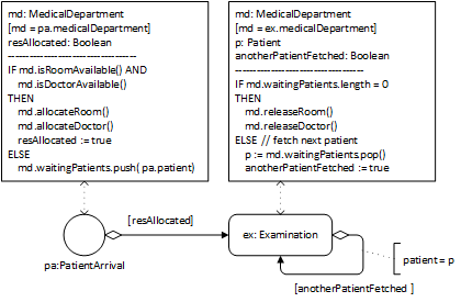
This process model defines the following two event rules.
| ON pa: PatientArrival |
|---|
| md : MedicalDepartment resAllocated : Boolean md := pa.medicalDepartment |
| IF md.isRoomAvailable() AND md.isDoctorAvailable() THEN md.allocateRoom(); md.allocateDoctor(); resAllocated := true ELSE md.waitingPatients.push( pa.patient); resAllocated := false |
| IF resAllocated SCHEDULE Examination( patient:=pa.patient, medicalDepartment:=md) |
| ON ex: Examination |
|---|
| md : MedicalDepartment anotherPatientFetched : Boolean p: Patient md := ex.medicalDepartment |
| IF md.waitingPatients.length = 0 THEN md.releaseRoom(); md.releaseDoctor(); anotherPatientFetched := false ELSE p := md.waitingPatients.pop(); anotherPatientFetched := true |
| IF anotherPatientFetched SCHEDULE Examination( patient:=p, medicalDepartment:=md) |
Notice that the event scheduling arrows of Figure 9-12, and also the SCHEDULE statements of the corresponding event rule tables, do not contain assignments of the duration of activities, since it is assumed that, by default, whenever an activity type has an operation duration(), the duration of activities of this type are assigned by invoking this operation.
A general model with resource objects as members of resource pools
In a more general approach, instead of using resource counter attributes, explicitly modeling resource object classes (like Room and Doctor) allows representing resource roles (stereotyped with «res») and resource pools (stereotyped with «pool») in the form of collections (like md.rooms and md.doctors) and modeling various forms of non-availability of resources (such as machines being defective or humans not being in the shift plan) with the help of corresponding resource status values (such as OUT_OF_ORDER). The result of this elaboration is the information design model shown in Figure 9-13.

For an OE class model, like the one shown in Figure 9-13, the following completeness constraint must hold: when an object type O (like Doctor) participates in a «res» association (a resource role association) with an activity type A (like Examination), the process owner object type of A (MedicalDepartment) must have a «pool» association with O.
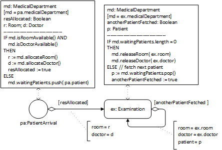
Extending OE Class Diagrams by adding a «resource type» category
The
information design model of Figure 9-13 contains two
object types, Room and Doctor, which are the range of resource
role and resource pool properties (association ends stereotyped «res» and
«pool»). Such object types can be categorized as «resource type» with the
implied meaning that they inherit a resource status attribute from a
pre-defined class Resource, as shown in Figure 9-16.
Resource
The introduction of resource types to OEM class models allows simplifying models by dropping the following modeling items from OE class models, making them part of the implicit semantics:
- the status attributes of object types representing resource types, which are implicitly inherited;
- the pre-defined enumeration ResourceStatusEL;
- the resource management operations isAvailable, allocate and release, which are implicitly inherited by any resource type; and
- the planned activity queues may possibly be implicitly represented for any resource-constrained activity type in the form of ordered multi-valued reference properties of its process owner object type.

Revisiting the manufacturing workstation example
A manufacturing workstation, or a "server" in the terminology of Operation Research, represents a resource for the processing activities performed at/by it. This was left implicit in the OE class model shown on the right-hand side of Figure 8-3. Using the new modeling elements (resource types, resource roles and resource pools), the processing activities of a workstation can be explicitly modeled as resource-constrained activities, leading to the OE class model shown in Figure 9-17 and to a more high-level and more readable process model compared to the process model of Figure 8-4.

Decoupling the allocation of multiple resources
In a simplified simulation design for the extended scenario (with patients and nurses first walking to examination rooms before doctors are allocated for starting the examinations) described by the conceptual models of Figure 9-6 and Figure 9-9, we do not consider the walks of doctors, but only the walks of nurses and patients. For simplicity, we drop the superclass people and associate the activity type WalkToRoom with the Patient and Nurse classes. The result of this elaboration is the information design model shown in Figure 9-18.

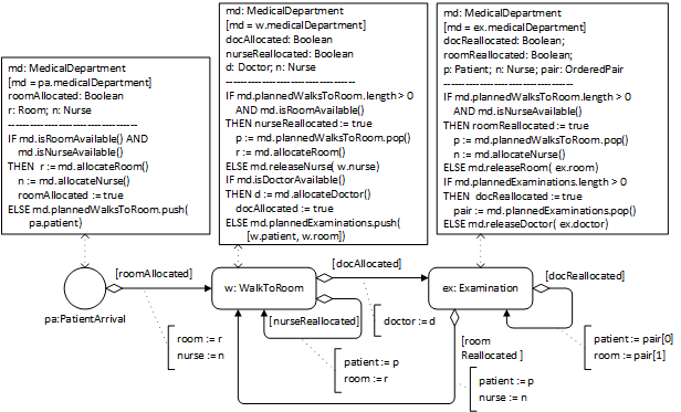
This process design model defines three event rules. Notice that the Examination event rule either re-allocates the doctor to the next planned examination and schedules it, if there is one, or it releases the doctor and re-allocates the room to the next planned walk-to-room and schedules it, if there is one.
Centralizing the re-allocation of resources
As shown before, in the conceptual process models of Figure 9-8 and Figure 9-9, the re-allocation of resources can be centralized with the help of resource release request events and the process owner and the involved performers can be displayed by using a Pool that is partitioned into Lanes for the involved activity performers, resulting in the model shown in Figure 9-20.
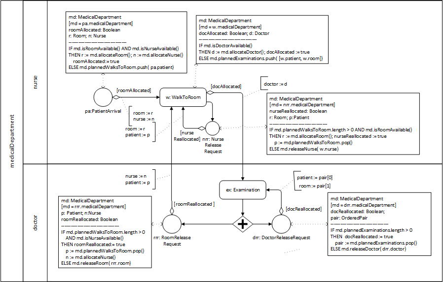
9.3. Introducing Resource-Dependent Activity Scheduling Arrows
The conceptual process model shown in Figure 9-9 and the process design model shown in Figure 9-20 exhibit a general pattern for modeling a sequence of two resource-constrained activities of types A1 and A2 shown in Figure 9-21. For describing this Allocate-Release Modeling Pattern, we assume that
- the process owner maintains queues for planned activities: q1 for for planned activities of type A1, and q2 for planned activities of type A2, both defined as queue-valued (i.e., ordered multi-valued) reference properties of the process owner in the underlying information model;
- the underlying information model specifies the sets of resources R1 and R2 required by A1 and A2;
- the set of resources required by A2 but not by A1 is denoted by R2−R1;
- the set of resources required by A1 and by A2 is denoted by R1∩R2.

We can describe the execution semantics of the Allocate-Release Modeling Pattern for the case of a succession of an activity of type A1 by another activity of type A2 in the following way:
- ON start event:
- If the resources R1 required by A1 are available, they are allocated; otherwise, a planned A1 activity is added to the task queue q1.
- If the resources R1 have been allocated, a new activity of type A1 is started.
- WHEN an activity of type A1 is
completed:
- If available, the resources R2−R1 are allocated; otherwise, a planned A2 activity with reserved resources R1∩R2 is added to the task queue q2.
- If R2−R1 have been allocated, a new activity of type A2 (with resources R2−R1 and R1∩R2) is started. In addition, the release of R1−R2 is requested.
- ON release request for
R1−R2:
- If q1 is not empty and the resources R1∩R2 required by both A1 and A2 are available, they are allocated and R1−R2 are re-allocated to head( q1); otherwise, R1−R2 are released.
- If the resources R1−R2 have been re-allocated, a new activity of type A1 is started.
- WHEN an activity of type A2 completes:
- There is no state change.
- An immediate release request for R2 is caused/scheduled.
- ON release request for R2:
- If R1∩R2 is nonempty: if q1 is not empty and the resources R1−R2 required by A1, but not yet allocated, are available, they are allocated and R1∩R2 are re-allocated to head( q1); otherwise, R1∩R2 are released. If q2 is not empty, then re-allocate R2−R1 to head( q2); otherwise, R2−R1 are released.
- If R1∩R2 have been re-allocated, a new activity of type A1 is started. If R2−R1 have been re-allocated, a new activity of type A2 is started.
Since the Allocate-Release Modeling Pattern defines a generic algorithm for scheduling resource-constrained activities as well as allocating and releasing resources, its (pseudo-)code does not have to be included in a DPMN Process Diagram, but can be delegated to an OE simulator supporting the resource-dependent scheduling of resource-constrained activities according to this pattern. This approach allows introducing new DPMN modeling elements for expressing the Allocate-Release Modeling Pattern in a concise way, either leaving allocate-release steps completely implicit, as in the DPMN Process Diagram of Figure 9-22, or explicitly expressing them, as in Figure 9-23.
The most important new DPMN modeling element introduced are Resource-Dependent Activity Scheduling (RDAS) arrows pointing to resource-constrained activities, as in Figure 9-22. These arrows are high-level modeling elements representing the implicit allocate-release logic exhibited in Figure 9-21. Thus, the meaning of the model of Figure 9-22 is provided by the model of Figure 9-21.

It is an option to display the implicit allocate-release steps with Allocate and Release rectangles together with simple control flow arrows, as between the start event circle and the Allocate R1 rectangle in Figure 9-23.

The meaning of the model of Figure 9-23 is the same as that of Figure 9-22, which is provided by the model of Figure 9-21. The fact that, using RDAS arrows, the allocate-release logic of resource-constrained activities does not have to be explicitly modeled and displayed in a process model shows the power of founding a process model on an information model, since the entire resource management logic can be expressed in terms of resource roles, constraints and pools in an information model. This is in contrast to the common approach of industrial simulation tools, such as Simio and AnyLogic, which require defining resource roles, constraints and pools as well as explicit allocate-release steps in the process model, in a similar way as shown in Figure 9-23.
The Standard Allocate-Release Algorithm
For each activity type, it has to be decided, if the resources required for a planned activity of that type are allocated at once or successively as soon as they become available. We call these two allocation policies Single-Step Allocation (SSA) and Multi-Step Allocation (MSA).
We can describe the Standard Allocate-Release Algorithm for the case of an event of type E succeeded by an activity of type A1 succeeded by another activity of type A2, with Ri and qi being the set of resource roles and the task queue of Ai, in the following way:
- WHEN an event e@t of type E occurs:
- A planned activity a of type A1 is created. If all R1 resources are available, they are allocated to a. Otherwise: (1) if MSA, then all available R1 resources are allocated to a; (2) a is added to the task queue q1.
- If all R1 resources have been allocated to a, it is started.
- WHEN an activity a1 of type
A1 is completed:
- A planned activity a2 of type A2 is created. If all R2−R1 resources are available, they are allocated to a2 and R1∩R2 are re-allocated from a1 to a2 (resulting in an allocation of all R2 resources to a2). Otherwise: (1) if MSA, then all available R2−R1 resources are allocated to a2 and R1∩R2 are re-allocated from a1 to a2; (2) a2 is added to q2.
- If all R2 resources have been allocated to a2, it is started. In addition, if MSA, the release of all R1−R2 resources is requested, else the release of all R1 resources is requested.
- ON release request for
R1−R2:
- If q1 is not empty and the resources R1∩R2 required by both A1 and A2 are available, they are allocated and R1−R2 are re-allocated to head( q1); otherwise, R1−R2 are released.
- If the resources R1−R2 have been re-allocated, a new activity of type A1 is started.
- WHEN an activity of type A2 completes:
- There is no state change.
- An immediate release request for R2 is caused/scheduled.
- ON release request for R2:
- If R1∩R2 is nonempty: if q1 is not empty and the resources R1−R2 required by A1, but not yet allocated, are available, they are allocated and R1∩R2 are re-allocated to head( q1); otherwise, R1∩R2 are released. If q2 is not empty, then re-allocate R2−R1 to head( q2); otherwise, R2−R1 are released.
- If R1∩R2 have been re-allocated, a new activity of type A1 is started. If R2−R1 have been re-allocated, a new activity of type A2 is started.
Since the Allocate-Release Modeling Pattern defines a generic algorithm for scheduling resource-constrained activities as well as allocating and releasing resources, its (pseudo-)code does not have to be included in a DPMN Process Diagram, but can be delegated to an OE simulator supporting the resource-dependent scheduling of resource-constrained activities according to this pattern. This approach allows introducing new DPMN modeling elements for expressing the Allocate-Release Modeling Pattern in a concise way, either leaving allocate-release steps completely implicit, as in the DPMN Process Diagram of Figure 9-22, or explicitly expressing them, as in Figure 9-23.
Connecting two Activity rectangles with an RDAS arrow in a DPMN process diagram implies DPMN's standard allocate-release algorithm according to which required resources that have not been allocated before are allocated immediately before an activity requiring them is started and released immediately after this activity is completed if they are not required by a successor activity. More precisely, when an activity of type A is completed, any resource that is not required by a successor activity of type B will be allocated to the next enqueued activity of type A, if there is one, or otherwise released.
Whenever another (non-standard) Allocate-Release logic is needed, it has to be expressed explicitly using conditional event scheduling arrows instead of RDAS arrows.
Example 1: Simplifying the workstation process model
We can now simplify the workstation model using the resource type category for WorkStation in the OE class model and a resource-dependent activity scheduling arrow from the arrival event to the processing activity in the DPMN process model. The resulting class model is shown in Figure 9-26.
The simplification of the process model of Figure 8-5 results in the model of Figure 9-25.

Example 2: Simplifying the medical department process model
We can now simplify the medical department model using the resource type category for Doctor, Room and Nurse in the OEM class model and resource-dependent activity scheduling arrows in the DPMN process model. The resulting class model is shown in Figure 9-26.
The simplification of the rather complex process model of Figure 9-20 by using resource-dependent activity scheduling arrows results in the model of Figure 9-27.

9.4. Organization Modeling Concepts
The activities of a business process are typically performed by human resources holding certain organizational positions that authorize them to play certain organizational roles within an organization or organizational unit. It is, therefore, natural that Activity-Based DES modeling includes organization modeling concepts. In particular, the concept of resource roles and the related concepts of organizational roles and organizational positions are paramount to Activity-Based DES modeling.
Many resource modeling concepts, such as resource roles (including performer roles) and resource pools, can be captured in information models in the form of categorized ("stereotyped") UML class modeling elements such as «rr» for resource role association ends, «pr» for performer role association ends, and «rp» for resource pool association ends, leading to an extension of UML Class Diagrams, called OE Class Diagrams, such as the following one:

This conceptual OE class model describes two activity types, "walks to rooms" and "examinations", each one associated with
- the object type "medical departments", providing the (business) process owner; implying that each specific walk-to-room or examination activity is performed by human resources of, and within a business process owned by, that department;
- a performer object type ("nurses" or "doctors") via a performer role («pr») association end, providing the activity performer (as a special type of resource);
- another resource object type via a resource role («rr») association end, providing another resource of each activity (a "room").
In addition, the model describes three types of resource pools by means of «rp» association ends, such that each resource pool is associated with a process owner maintaining the pool and providing the resources corresponding to one of the three resource roles.
Notice that in a conceptual OE class model, each activity type should have a performer role («pr») association, while in an OE class design model (being part of a simulation design model), it is an option to abstract away from the distinction of performers among the resources of an activity and simply consider all its resources (including its performer) as plain resources. This is common in management science and Operations Research, where the main interest is in obtaining general performance statistics for resources, such as their utilization, no matter if they are active resources (performers) or not.
We show how further organization modeling concepts can be introduced to OEM&S.
Refining Object Types to Resource (Role) Types and Performer (Role) Types
While a resource role of an activity type denotes an association end, corresponding to a reference property of the class implementing the activity type, a resource (or performer) role type denotes an object type that is the range of a resource (or performer) role. For simplicity, we say "resource type" (or "performer type") instead of "resource role type" (or "performer role type").
For all «object type» classes of an OE class model that are the range of a performer role or a resource role, it may be an option to replace their «object type» category with a «performer type» or «resource type» category, as shown for the object types "nurses", "doctors" and "rooms" in the following refined model:

Notice that typically each resource type is the range of one resource role and represents a resource pool for it. A resource type may be the target class of more than one resource role association end and its population may be segmented into several resource pools such that at least one pool is assigned to each resource role.
However, the replacement of the «object type» category of a class with a (performer or resource) role type category is only an option, if all instances of the class are playing that role. In the above example, if there are doctors who do not perform examinations (but only surgical operations), then the object type "doctors" cannot be turned into a performer type "doctors" for examinations, but would have to be partitioned into two subtypes, "surgeons" and "examination doctors", such that the latter would be a performer type for examinations.
In OEM&S, a human performer type is implicitly a subtype of the pre-defined object type Person. This makes it possible that a doctor, as a person that performs examinations, may also be a patient in an examination (of course, with the constraint that a person cannot be the same examination's doctor and patient).
Refining Performer Types to Organizational Positions
An organizational position is defined by a name and a set of human performer types representing the roles of the position holders. For instance, in a medical department, the organizational position Nurse may be defined by the set of performer types Guide and ExaminationAssistant, where a Guide is required for guiding a patient to an examination room and an ExaminationAssistant is required for assisting a doctor in a medical examination.
Computationally, an organizational position is an object type that is co-extensional with all of its performer types, implying that its instances (position holders) are human resources that can be allocated for performing any activity associated with any of these performer types. This implies that any instance (or "holder") of an organizational position is a person and that any organizational position is a subtype of the kind Person.
For instance, the organizational position Nurse is co-extensional with the performer types Guide and ExaminationAssistant, with the meaning that nurses may play the role of guides or the role of examination assistants, and any guide, as well as any examination assistant, is a nurse.
In simple cases, an organizational position is defined by just one performer type for one particular performer role.
In OEM&S, for each organizational position (like Clerk) consisting of the performer roles p1,...,pn, there is a default resource pool, or better: performer pool, (like clerks) that includes all employees holding that position. This pool will be used for allocating the performers of activities with a performer role pi.
These considerations lead to the following refined version of the medical department model shown in the diagram above:

Notice that in this refined model, we have also categorized the object type "patients" as «person role type» and the object type "medical departments" as «organizational unit type». In OEM&S, a person role type, like Patient, is implicitly a subtype of the pre-defined object type Person, allowing a doctor to be a patient. An organizational unit, as an instance of an organizational unit type, may own one or more business processes.
Assigning business process types and business goals to organizational agents
An organizational agent, which is either an organization, an organizational unit or an organizational role player, can own business process types and can have business goals, which allow improving business processes by refactoring business process models, including resource allocation policies, and by changing the populations of resource pools, in such a way that the goals of the process owner (and those of its super-agents) are satisfied.
Consider the following example:
A business company has a Marketing department owning a Lead Generation process, a Business Development unit owning a Lead Qualification process, a Sales department owning a Sales process and a Customer Success department owning a Customer Success process. The company has the overall top-level goals "increase profit", "increase customer satisfaction", and "increase employee motivation".
Without the overall company goals in mind, each organizational unit is prone to optimize their subprocess without keeping an eye on the long-term implications:
- Marketing maximizes lead output and ignores that most leads it generates won’t be qualifiable.
- In its struggle to identify high-quality leads in a mass of low-quality lead data, Business development is overly eager to interpret leads as ‘qualified’, even if it is clear that many leads they forward to Sales can’t be turned into long-term customers.
- Sales tries to close as many deals as possible, without considering churn and missed up-sell opportunities if the product can’t deliver on the promises made.
- Customer success can’t do more than fight the fires of customer dissatisfaction.
This behavior is often encouraged by middle management that sets simple and easily quantifiable short-term performance goals for the team that reports to them, without keeping the big picture in mind.
There are different ways of expressing business goals. In simulation modeling, we need operational forms of business goals, that is, expressions in a formal language. We consider three forms of business goals:
- Definite goals (like "raise the overall revenue by at least 25%") are defined by a logical condition (like relativeRevenueRise >= 0.25) that can be checked by a simulator.
- Variable change goals are defined by a combination of one of the verbs "increase" or "decrease" with the name of a variable (like "profit", "customer satisfaction" or "costs").
- Optimization goals are (more ambitious) special variable change goals defined by a combination of one of the verbs "maximize" or "minimize" with the name of a variable (like "profit", "customer satisfaction" or "costs").
9.5. Resource Modeling
Whenever an activity of a certain type is to be performed, various resources may be required for performing it and have to be allocated first. We can distinguish between ‘active’ (or performer) resources, such as human resources, robots or IT systems, which execute activities, and ‘passive’ resources, such as rooms or devices, which are used by performers for executing activities.
Business process models focus on describing the possible sequences of events and activities, based on conditional and parallel branching. But they may also describe resource roles, which associate resources of a certain type with activities of a certain type.
In the field of Business Process Management (BPM), there is a tendency to consider workflow processes as paradigmatic for business processes. However, workflow processes typically only have (human) performer resources, while business processes in general often have one or more passive resources in addition to a performer. Due to this tendency, BPM research often adopts a simplistic view of business processes.
E.g., in (Pufahl et al. 2021), resource allocation is defined as the “assignment of a process task to the most appropriate resource”, while in general, it’s the other way around: resources are assigned to a task. The authors also point out that the vast majority of BPM research studies on resource allocation make the assumption that a task requires just one resource and a resource cannot be used in more than one task at the same time. As opposed to this simplistic view of business processes in BPM, in DES, tasks can have more than one required resource, and resources may be used in more than one task at the same time.
It is important to distinguish between the passive resources required for performing an activity and the inputs required for performing a processing (or transformation) activity. While the passive resources used in an activity survive the activity, and can be reused in the next one, inputs are either processed, or transformed, into outputs of the activity, and cannot be reused for the next activity. In the literature, this conceptual distinction is often not made. Instead, e.g., in (Russell et al. 2004; Goel and Lin 2021), processing activity inputs are called ‘consumable resources’. However, resources cannot be ‘consumed’, but they can be worn out by activities, such that if their degree of wear falls below a certain threshold, they can no longer be used and are depleted.
For various reasons, resources can go out of order: machines may fail or may have to get scheduled maintenance, nurses or doctors may get sick or may be out-of-duty or off-shift. Consequently, both planned and unexpected resource outages may have to be modeled.
9.5.1. Resource Cardinality Constraints and Multitasking Constraints
Since activities require resources, and resources are allocated to planned activities, it is crucial to understand the relationship between activities and resources. An important part of its meaning are resource cardinality constraints and multitasking constraints.
Business process models do not only describe the possible sequences of events and activities, but they also describe the dependency of activities on resources. For instance, in a BPMN process diagram, a Lane L (such as the doctors lane in the BPMN process diagram below) may represent a resource type such that the diagram specifies for any Activity rectangle A in L (such as examinations) that an activity of type A is performed by a resource of type L.

While using a container shape, such as a BPMN Lane, for assigning elements, such as activities, to the element represented by the container shape (viz, a resource role) is a good way of visually expressing a many-to-one relationship between activity types and resource roles (all activity types within a Lane do have exactly one resource role), it does not allow expressing one-to-many or many-to-many relationships between activity types and resource roles.
Therefore, the BPMN Lane notation can only be used for specifying a performer resource role for activities that do not require resources of other types, and where we have a one-to-one association: (1) a resource can be allocated to at most one activity, and (2) an activity is performed by exactly one resource.
In general, though, the relationships between activities (of some type) and resources (of some type) can be best described by binary relationship types in an information model, such as by binary associations in a UML class diagram with multiplicity expressions at both ends. Figure 9-29 shows two one-to-one associations between the activity type examinations and the object types rooms and doctors associating a room as a (passive) resource and a doctor as a performer resource to an examination activity.

The association end at the side of the object type doctors is categorized as a resource role with the help of UML’s stereotype notation. The multiplicity expression at the resource role end is called resource multiplicity. In our example, the resource multiplicity at the doctors end is ”1” (an abbreviation of "1..1"), which means that exactly one doctor is required for performing an examination, defining a resource cardinality constraint that is a conjunction of a minimum resource cardinality constraint ("at least one") and a maximum resource cardinality constraint ("at most one").
In general, a multiplicity expression defines both a lower bound and an upper bound. When the lower bound of a resource multiplicity is greater than 0, it defines a minimum resource cardinality constraint. When the upper bound of a resource multiplicity is a natural number greater than 0, it defines a maximum resource cardinality constraint. The resource multiplicity 0..* (where * stands for unbounded), which does not define any resource cardinality constraint, is rather unusual since normally all activities require at least one resource (their performer).The multiplicity of the association end at the other side (of the activity type) represents a multitasking constraint, which defines if a resource is exclusively allocated to an activity, or to how many activities a resource can be allocated at the same time. In our example, the multiplicity 0..1 represents a multitasking constraint stating that, at any point in time, a doctor can be associated with, or perform, either no examination or at most one examination.
In an Object-Oriented (OO) programming approach, the computational meaning of a resource role is provided by a corresponding property in the class implementing the activity type. In the above example, the resource role association of "examinations" with "doctors" leads to a property doctor in the class Examination, as shown in Figure 9-30.
When activities admit using more resources than required, this means they can be started as soon as the required number of resources are available, but they can also be started with a greater number of resources, typically implying a faster performance.

While the model shown in Figure 9-29 is an example of a one-to-one association between an activity type and a resource object type, which is the only option in BPMN process models, we consider the cases of one-to-many, many-to-one and many-to-many associations in the following subsections.
One-to-Many Relationships
An example of a one-to-many relationship between activity types and resource object types is the association between ”load truck” activities and ”wheel loader” resources shown in Figure 9-31.

Notice that in this diagram, the «resource role» designation of the association end at the side of “wheel loaders” has been abbreviated by the keyword «rr». Its resource multiplicity of 1..2 specifies a minimum resource cardinality constraint of “at least one” and a maximum resource cardinality constraint of “at most two”, meaning that one wheel loader is required and a second one is admissible. When an activity does not require, but admits of, using more than one resource (of the same type), this typically means that the duration of the activity is the more decreasing the more resources are being used.
The one-to-many resource role association of ”load truck” with ”wheel loaders” leads to a property wheelLoaders in the activity class LoadTruck, as shown in Figure 9-32. Notice that this property has the multiplicity 1..2, which means that it is collection-valued and has either a singleton or a two-element collection value.

When activities admit using more resources than required, this means they can be started as soon as the required number of resources are available, but they can also be started with a greater number of resources, typically implying a shorter duration.
Many-to-One Relationships
An example of a many-to-one relationship between activity types and resource object types is the association between ”examination” activities and ”examination room” resources shown in Figure 9-33.

In this example, examination rooms (as resources) admit of up to three examinations being performed at the same time. Such a multitasking constraint can be implemented with the help of a (multitasking) capacity attribute of the class implementing the resource object type. If such a constraint applies to all instances of a resource object type, capacity would be a class-level (”static”) attribute, which is rendered underlined in a UML class diagram, as shown in the following model:

Alternatively, if different examination rooms have different capacities, then capacity would be an ordinary (instance-level) attribute of the class ExaminationRoom.
Many-to-Many Relationships
Examples of many-to-many relationships between activity types and resource object types are rare and typically involve activities going on with interruptions. An example is the association between ”teaching a course” activities and ”teacher” resources shown in Figure 9-34. In this example, the teaching of a course admits at most two teachers who may be involved in at most 7 course teaching activities at the same time.

9.5.2. Organizational Positions and Resource Pools
Since a business process happens in the context of an organization, it is natural to consider the concept of organizational positions, which has been introduced in Section 9.4.
Resource roles (including performer roles), resource types (including performer types), organizational positions and resource pools are defined in an OE class model. A resource role of an activity type is a special type of property having a resource type as its range.
A performer role of an activity type has a performer type as its range. For instance, in the following OE class model, the (implicitly named) performer role orderTaker of the activity type TakeOrder has the performer type OrderTaker as its range. Likewise the object type PizzaMaker is a performer type. A performer type may be an organizational position. For instance, in the following OE class model, both OrderTaker and PizzaMaker are organizational positions, for which an organization hires a number of human resources, forming corresponding resource pools (called orderTakers and pizzaMakers). These resource pools correspond to the direct populations of the two organizational positions.

An organizational position may subsume more than one performer role. In the model above, the organizational position PizzaMaker is an alternative resource subtype of the organizational position OrderTaker, as indicated by the generalization arrow with the category keyword «ar» (a UML "stereotype").
When a resource pool represents an organizational position charged with playing n performer roles, it is used by all n corresponding activity types.
It is an option that the resources of an alternate resource pool, corresponding to an alternative resource subtype, are associated with a lower proficiency level increasing both the duration of activities and their rework probabilities.
9.5.3. Alternate Resource Pools
Certain activities allow alternative resources, when no standard resources are available. For instance, in a pizza service company, when no order taker is available, and a new order call comes in, an available pizza baker can take the order. Or in a hospital, where nurses guide patients to an examination room, when no nurse is available, a receptionist can guide a patient to an examination room.
The general conceptual pattern is that for certain types of activities A (like GuideToRoom), a resource role r (like guide) may be played not only by instances of its direct resource type R (like Guide), but also by instances of an alternative resource type R' (like ExaminationAssistant) or an organizational position P (like Nurse), if they are a subtypes of R (Guide).
When the resource type R is not abstract, then its instances are the preferred resources of activities of type A, and its (possibly preference-rank-annotated) alternate resource subtypes specify types of alternative resources.
By default, for any non-abstract resource type R and for any organizational position P assigned as the range of a resource role r, an OE simulator can create a resource pool with the same (yet pluralized) name, pooling objects instantiating R or P, and assign it to r as the preferred resource pool.
An alternate resource pool can be defined in an OE class model by means of an alternate resource subtyping arrow (a UML generalization arrow designated with «ar») between the alternative resource type and the resource type concerned as shown in the following diagram, where PizzaMaker is modeled as an alternative resource subtype of OrderTaker:
9.5.4. Task Priorities
Whenever an activity of type A1 ends and there is still another A1 task in the queue, the activity's resources would be re-used for the next A1 task unless there is another task (say, of type A2) with higher priority waiting for one of the resources (r1). In that case, r1 is allocated to that task, and all other resources are allocated to the next A1 task, which still has to wait for r1 becoming available again.
For example, in a pizza service, where incoming orders can be taken by pizza makers, and TakeOrder tasks have a higher priority than MakePizza tasks, when a MakePizza activity performed by a pizza maker in an oven ends while there is still another MakePizza task in the queue and there is also a TakeOrder task in the queue, the pizza maker is allocated to the TakeOrder task and the oven is allocated to the next MakePizza task, which has to wait for a pizza maker becoming available.
Algorithmically: Whenever an activity a1 of type A1 ends, collect all pairs <r, t> such that r is a resource used by a1 and t is the next task of an activity type A from the dependent activity types DAT of pool(r) with the highest priority among all DAT with task priorities higher than A1. For all these pairs <r, t>, allocate r to t. Allocate the remaining resources of a1 to the next A1 task, if there is any, otherwise release them.
9.5.5. Activity Preemption
An ongoing activity may be preempted by a higher-priority task requiring a resource used by the ongoing activity. In such a case, the activity is either aborted or suspended, and the required resource is released from it and allocated to the higher-priority task. A suspended activity may be later resumed when a resource of the required type becomes available again.
9.5.6. Resource Outages
For various reasons, resources can go out of order: machines may fail or may have to get scheduled maintenance, nurses or doctors may get sick or may be out-of-duty or off-shift. Consequently, both planned and unexpected resource outages may have to be modeled.
While human resources being out-of-duty or off-shift can be modeled with the help of service time calendars, scheduled maintenance may be modeled in the form of maintenance activities recurring with a fixed interval. Unexpected resource outages are resource failures.
Modeling Resource Failures
Resource failures can be modeled with the help of two types
of events: failure and recovery, and two related random
variables: time-to-next-failure and failure time. In this
approach, the next resource failure event occurs x time units after a
recovery event, where x is obtained by invoking the random variable
sampling function timeToNextFailure(). Each failure event
triggers a recovery event, which is scheduled with a delay of y time
units where y is obtained by invoking the random variable sampling
function failureTime().
This simple approach applies both to non-human and human resources.
Further modeling options:
- Allow specifying a time-to-first-failure, in addition to the time-to-next-failure.
- Allow counting only the busy time of a resource, instead of the total time, for determining its next failure time.
Modeling the Repair of Failed Resources
In activity-based simulation, the basic failure modeling approach can be refined by modeling the repair of a failed non-human resource as an activity whose duration is provided by the random variable repair time and which requires a repair person as a resource, such that the total failure time is the sum of the two random variables repair lead time (the time needed for getting a repair person to start the repair) and repair time.
Then, when a failure event occurs, it triggers a
repair activity to start with a delay of x time units and a
duration of y time units, where x =
repairLeadtime() and y = repairTime(). The
next failure event is scheduled to occur z time units after a
repair end event, where z is obtained by invoking the random
variable sampling function timeToNextFailure().
Modeling the Scheduled Maintenance of Resources
Non-human resources, such as
machines, may undergo periodic maintenance for preventing them to fail in
the near future. This can be modeled by scheduling periodic
maintenance activities every x time units where x =
maintenanceIntervall(), along with periodic failure events.
When a maintenance activity starts before the next scheduled
failure event has occurred, the simulator has to retract this event
from the Future Event List for implementing its prevention by the
maintenance activity. The next failure event is scheduled to occur
x time units after the maintenance end event, where
x is obtained by invoking the random variable sampling function
timeToNextFailure().
When a resource fails before its
next scheduled maintenance has started, the scheduled
maintenance is cancelled (the simulator has to retract the
scheduled maintenance start event) and, instead, the
failure event triggers a repair activity. Only when the
repair activity ends, the next maintenance activity is
scheduled with a delay of y time units where y is obtained by
invoking the random variable sampling function
maintenanceTime().
Further modeling options:
- Allow specifying a time-to-first-maintenance, in addition to the maintenance interval time-to-next-maintenance.
- Allow specifying the recurrence of maintenance activities with a schedule instead of a (typically fixed) maintenance interval.
Defining General Elements for Modeling Resource Outages
A simulation framework/language should support resource outage modeling by allowing to define for each (non-human) resource object type the three pairs of (typically random variable) time functions introduced above and summarized in the following class diagram.

These pairs of time functions have to be used incrementally: specifying maintenance time functions requires specifying repair time functions, which, in turn, requires specifying failure time functions.
Resource Outage Modeling in AnyLogic
AnyLogic is a state-of-the-art DES modeling tool/framework. It allows defining recurrent failures (not with follow-up recovery events, but only with follow-up repair activities) and maintenance for each Resource Pool. There is the option to use only the busy time of a resource for computing its next failure time. For repair activities, there is no possibility to distinguish between repair lead time and repair time. For maintenance activities, it can be defined which task priority they have and if they are preemptive or not. Neither for repair nor for maintenance activities, performer resources can be assigned.
9.6. The AN Formalism
Formally, an AN is defined on the basis of a set of object types OT, a set of event types ET and a set of activity types AT as a directed graph ⟨ N, D ⟩ with two types of nodes N = EN ⋃ AN, event nodes and activity nodes, and two types of directed edges D = ED ⋃ AD, event scheduling edges and resource-dependent activity scheduling edges, with ED ⊆ N ⨉ EN and AD ⊆ N ⨉ AN, such that
each event node n ∈ EN is associated with
- an event type E ∈ ET with event participation roles PE,
- an event variable e representing an event of type E,
- a (possibly empty) set of auxiliary (shortcut) object variables o defined with the help of event participation roles p ∈ PE by setting o := e.p,
- a (possibly empty) set of definitions of on-event object state transition functions { fp | p ∈ PE };
each activity node n ∈ AN is associated with
- an activity type A ∈ AT with activity participation roles PA,
- an activity variable a representing an activity of type A,
- a (possibly empty) set of auxiliary (shortcut) object variables o defined with the help of activity participation roles p ∈ PA by setting o := a.p,
- a (possibly empty) set of definitions of on-activity-start object state transition functions { sfp | p ∈ PE };
- a (possibly empty) set of definitions of on-activity-end object state transition functions { efp | p ∈ PE };
- each event scheduling edge ⟨ n1,
n2 ⟩ ∈ ED may be associated with
- a numeric delay expression δ possibly expressed with the help of the variables associated with n1,
- a condition (or Boolean expression) C expressed with the help of the variables associated with n1.
Chapter 10. Case Studies
10.1. Make and Deliver Pizza

A pizza service company takes phone orders for making and delivering pizzas, with the help of order takers, pizza makers, ovens and a crew of pizza delivery scooter drivers. From time to time the order takers cannot cope with the number of incoming calls, and then customers grow impatient and hang up the phone without placing an order.
For getting a quick impression, you can run this model from the Sim4edu website, or inspect its OESjs code.
Since there is a high number of lost orders due to long waiting times in the first model, assigning different responsibilities to organizational roles for allowing a more flexible use of human resources is considered in a variant of the first model.
Our Make-and-Deliver-Pizza modeling problem is based on the chapter "Example Model 3: Pizzeria operation" in the book The Art of Process-Centric Modeling with AnyLogic by Arash Mahdavi.
Conceptual Model
A pizza service company has resource pools for order takers, pizza makers, pizza ovens, delivery staff and scooters. While take order activities are performed by an order taker, make pizza activities require both an oven and a pizza maker. Finally, deliver pizza activities require a delivery staff member and a scooter.
Conceptual Information Model
The potentially relevant object types are:
- pizza service company,
- customers,
- orders,
- pizzas,
- order takers,
- pizza makers,
- pizza ovens
- delivery scooter drivers,
- scooters.
Potentially relevant types of events and activities are:
- pizza ordering calls coming in from customers,
- order taking (an activity performed by order takers),
- customers hanging up the phone when having to wait for too long,
- pizza making (performed by pizza makers using ovens),
- pizza delivery (performed by delivery staff using scooters).
Object, event and activity types, together with their participation associations, can be visually described in a conceptual information model in the form of a special kind of UML class diagram, called Object Event (OE) class diagram, as shown below.

The association end annotations «rr» and «rp» denote resource roles and resource pools. For instance, the activity type make pizza has two resource roles, pizza makers and oven. A pizza service company has resource pools for order takers, pizza makers, ovens, delivery scooter drivers and scooters.
Resource roles have resource cardinality constraints. For instance, a make pizza activity requires 2 pizza makers and 1 oven.
A conceptual OE class diagram like the one above, describes resource roles (like oven), resource role types (like ovens) and resource cardinality constraints (like "exactly 1") for all types of activities.
An organization defines organizational positions, which are filled by human resources. Each organizational position is characterized by a set of human resource roles to be played by position holders. In the Pizza Service organization, there are three positions: order takers, pizza makers and delivery scooter drivers.
Strictly speaking, order phone calls are instantaneous (zero duration) events while a take order activity is an event with a non-zero duration. For simplicity, though, we'll often say "events" instead of "instantaneous events" or "objects, events and activities" instead of "objects, instantaneous events and activities".
Conceptual Process Model
The following BPMN diagram shows a conceptual process model of the Make-and-Deliver-Pizza business process, with three swimlanes for the three performers of the process:

Notice the BPMN Boundary Timeout Event circle attached to the take order activity representing timeout events that cancel the activity. They are supposed to model the reneging behavior of waiting customers loosing their patience and hanging up the phone without placing an order. However, BPMN does not allow restricting such a timeout mechanism to the waiting phase of a planned activity, that is the time span during which the planned activity has been enqueued, but not yet started. Rather, it applies to the entire cycle time of take order activities, which means that also started activities, where the order taker is already listening to the customer, may be canceled due to reneging.
While BPMN allows modeling the performers of activities with swimlanes, it does not support modeling other types of resource objects. As a workaround, we have included the resource objects ovens and scooters in the form of BPMN Data Objects.
The third, and most severe, issue of the BPMN model is its uniform (semantically overloaded) use of "sequence flow" arrows for sequencing events and activities. While in the case of all three activities, incoming "sequence flow" arrows do not mean that an activity is started, but rather that a new planned activity is enqueued (and only started when all required resources become available), in the case of the event lost order, the incoming "sequence flow" arrow means that a new event is scheduled to occur immediately.
These three issues of BPMN have been solved in DPMN, where resource-dependent activity scheduling (RDAS) arrows are distinguished from event scheduling arrows, as shown in the following DPMN process diagram:

Notice how the timeout event circle (with a clock icon) is attached to the three bars of the RDAS arrow representing the queue of planned order taking activities waiting for the availability of an order taker. This implies that the timeout applies to the waiting phase only, and not to the entire order taking activity.
A conceptual DPMN process diagram does normally not include any element representing a resource pool. Yet, it may display the performer roles of activity types, like order taker and pizza maker in the diagram above. It is assumed that for any organizational position described in the underlying OE class model, the organization under consideration has a corresponding resource pool.
Simulation Design
In our simulation design, we make the following simplifications. We consider only one particular pizza service company, which does not have to be modeled as an explicit object. Also, we abstract away from individual customers, orders and pizzas. And we merge the resource roles delivery scooter driver and scooter, keeping only scooters as resources of deliver pizza activities.
We consider a scenario with two order takers, ten pizza makers, five ovens and 20 scooters.
Information Design Model
An information design model, in the form of an OE class diagram as shown below, is derived from a conceptual information model by
- Abstracting away from items that are not design-relevant.
- Adding properties, functions and methods to object, event and activity classes. In particular, a status attribute is added to all resource object types, such as OrderTaker and Oven, and a class-level duration function is added to all activity classes.
Notice how functions representing random
variables, like the duration function of all activity types,
are marked with the keyword (or UML 'stereotype') «rv» standing for "random
variable". These random variable functions sample from a probability
distribution function (PDF), which is symbolically indicated with
expressions like Tri(30,40,50) standing for the triangular
PDF with lower and upper bounds 30 and 50 and a median of 40, or
DU(1,4) standing for the discrete uniform PDF with lower and
upper bounds 3 and 6.
In the case of the event type OrderCall, the random variable function recurrence samples from an exponential PDF with five different event rates given for the five consecutive hours during which the pizza service operates.
The activity type TakeOrder is associated with the object type OrderTaker via the implicit resource role orderTaker (with a resource cardinality constraint of "exactly 1"), indicated with the association end stereotype «rr» standing for "resource role". A resource role assigns resource objects to activities.
Likewise, MakePizza is associated with PizzaMaker and Oven via the (implicitly named) resource roles pizzaMakers, having a resource cardinality constraint of "exactly 2", and oven, having a resource cardinality constraint of "exactly 1".
An OE class design diagram like the one above, defines resource roles (like pizzaMakers), resource role types (like PizzaMaker) and resource cardinality constraints (like "exactly 2") for all types of activities. Normally, in an OE simulation there is a one-to-one correspondence between resource role types and resource pools. By convention, a resource pool has the same name as the corresponding resource role type, yet pluralized and starting with a lowercase character. For instance, the name of the resource pool for PizzaMaker is pizzaMakers.
Notice that OrderCall events are exogenous, having a recurrence function defined case-wise for each of the five hours per day operation of the pizza service company (in the attached invariant box).
For implementing the waiting timeout event defined in the process model, the activity type TakeOrder has a class-level waitingTimeout function implementing a random variable with PDF U(3,6).
Process Design Model
A process design model, in the form of a DPMN process diagram as shown below, is derived from a conceptual process model by abstracting away from items that are not design-relevant and possibly adding certain computational details.
A DPMN process design model (like the one shown in Figure 10-2) essentially defines the admissible sequences of events and activities together with their dependencies and effects on objects, while its underlying OE class design model (like the one shown in Figure 10-1) defines the types of objects, events and activities, together with the participation of objects in events and activities, including the resource roles of activities, as well as resource cardinality constraints, parallel participation constraints, alternative resources, and task priorities.
It is an option, though, to enrich a DPMN process design model by displaying more computational details, especially the recurrence of exogenous events, the duration of activities and the most important resource management features defined in the underlying OE class design model, such as resource roles (in particular, performer roles can be displayed in the form of Lanes) and resource cardinality constraints. The following model shows an enriched version of Figure 10-2:
Such an enriched DPMN process design model includes all computational details needed for an implementation without a separate explicit OE class design model. In fact, such a process model implicitly defines a corresponding class model. For instance, the enriched DPMN model of Figure 10-3 implicitly defines the OE class model of Figure 10-1 above.
The notation for defining performer roles in Lanes consists of a performer role name (such as pizzaMakers) and and an object type name (such as PizzaMaker) denoting its range, separated by a colon. When the performer role name is appended by a multiplicity expression in brackets, as in pizzaMakers[2], this denotes a resource cardinality constraint (stating that exactly 2 pizzaMakers are required). When only a performer type prefixed with a colon (such as :OrderTaker) is provided, this means that the implicit performer role name is obtained by lowercasing the performer type name (as in orderTaker:OrderTaker).
The notation for defining a non-performer resource role, such as oven:Oven, consists of a named object rectangle, such as the :Oven rectangle in Figure 10-3, attached to an activity rectangle by means of a connection line with a small filled square representing a resource link, such as the line between the MakePizza activity rectangle and the :Oven object rectangle in Figure 10-3.Notice that the model of Figure 10-3 does not include any element representing a resource pool. It is assumed that for any organizational position described in the underlying OE class model, the organization under consideration has a corresponding resource pool. By default, each resource role of an activity type is associated with a resource pool having the same (yet pluralized) name, such that its resource objects are instances of a corresponding resource role type, which is an organizational position in the case of human resources.
For instance, for the MakePizza activity a pool ovens is assigned to its resource role oven by default. The members of the pool ovens are instances of the (resource) object type Oven. Likewise, a pool pizzaMakers is assigned to the MakePizza resource role pizzaMaker. The members of this pool are instances of the organizational position PizzaMaker. These default pool assignments are normally not shown in a DPMN diagram, but an OE simulator takes care of them.
Combined with its underlying OE class design model, a DPMN process design model provides a computationally complete specification of a simulation model that can be directly turned into implementations.
Model Variant: Orders May Also Be Taken by Pizza Makers
For decreasing the number of lost orders due to long waiting times, it is advisable to charge pizza makers with taking orders whenever no order taker is available. In resource management terminology, the organizational position pizza maker is redefined by adding the performer role order taker to its portfolio of organizational roles.
In an OE class diagram, this can be expressed by adding a subtyping arrow from pizza makers to order takers categorized as an alternative resource subtyping arrow with the stereotype «ar», as shown in the following diagram:

The DPMN process model is not affected by this change.
10.1.1. Implementation with OESjs
The JavaScript-based simulator OESjs-Core2 implements the Object Event Simulation (OES) paradigm, and, consequently, allows a straight-forward coding of OE class models and DPMN process models.
Implementing the
Information Design Model
For implementing the OE class design model with OESjs-Core2, we have to code all object types, event types and activity types specified in the model in the form of JavaScript classes extending the respective OESjs framework classes oBJECT, eVENT and aCTIVITY. We start with the object type OrderTaker shown in the following diagram:

The OrderTaker object class can be
coded in the following way:
class OrderTaker extends oBJECT {
  constructor({ id, name, status}) {
    super( id, name);
    this.status = status;
  }
}
All object classes inherit an id attribute and a
name attribute from the pre-defined OES foundation class
oBJECT. Since order takers are resource objects, we need to
define a status property having the pre-defined enumeration
data type ResourceStatusEL as its range.
The other object classes (PizzaMaker, Oven and Scooter) are coded in the same way.
We next show how to code the event type OrderCall depicted in the following diagram:

The OrderCall event class is coded in
the following way:
class OrderCall extends eVENT {
  constructor({ occTime, delay}) {
    super({occTime, delay});
  }
  createNextEvent() {
    return new OrderCall({delay: OrderCall.recurrence()});
  }
  static recurrence() {
    var hour = Math.floor(sim.time / 60);
    return rand.exponential( OrderCall.arrivalRates[hour]);
  }
}
// arrival rates per minute (for a daily operation for 5 hours)
OrderCall.arrivalRates = [1/6, 1/0.66, 1/1.5, 1/6, 1/12];
All
event classes inherit an occTime attribute and a
delay attribute from the pre-defined OES foundation class
eVENT. Any event in OES can be created either with a
value for the attribute occTime (standing for occurrence
time) or with a value for the attribute delay. In the
latter case, the event's occurrence time is automatically derived by adding
the value of delay to the current simulation time.
Notice how the time-varying recurrence rates (representing order
arrival rates) are implemented in the recurrence function: by
first computing the current hour, which is then used as an index for
accessing the corresponding element of the
OrderCall.arrivalRates array.
Finally, we show how to code the activity type TakeOrder depicted in the following diagram:

The TakeOrder activity class is coded in the following way:
class TakeOrder extends aCTIVITY {
  constructor({id, startTime, duration}={}) {
    super({id, startTime, duration});
  }
  static duration() {
    return rand.uniform( 1, 4);
  }
  static waitingTimeout() {
    return rand.uniformInt( 3, 6);
  }
}
TakeOrder.resourceRoles = {
  "orderTaker": {range: OrderTaker}
}
All activity classes inherit the attributes id,
startTime and duration from the pre-defined OES foundation class
aCTIVITY. When an activity is created as a JS object during a
simulation run, the value of its duration property is obtained
by invoking the duration() function defined as a class-level
("static") function for its activity class. These activity duration
functions typically implement a random variable by invoking a random variate
sampling function, such as rand.triangular(30,50,40), which
samples from the triangular probability distribution function (with
min/max=30/50 and mode=40).
Notice how the resource role association
between TakeOrder and OrderTaker, which defines the resource
reference property TakeOrder::orderTaker, is coded by a corresponding
entry in the map-valued class-level property
resourceRoles.
Implementing the Process Design
Model
The following process design model specifies six types of events: order call events, take order waiting timeouts, lost order events, take order activities, make pizza activities, and deliver pizza activities:
A DPMN process design model can be decomposed into
a set of event rule design models, one for each type of event specified in
the design model. Since the LostOrder event and the
DeliverPizza activity do not have any effects, we only need
four event rules.
1 The OrderCall event
rule
Starting with the following OrderCall event rule
design model, we show how the event rules specified by each of these event
rule design models can be coded.

The
OrderCall event rule does not define any state changes of
affected objects, but only the resource-dependent scheduling of a
TakeOrder activity, which is coded with the following OESjs
statement:
OrderCall.successorActivity = "TakeOrder";
2
The TakeOrder Waiting Timeout event rule

The TakeOrder Waiting Timeout event
rule only schedules the immediate occurrence of a LostOrder
event, which is coded with the following OESjs event routine within the
TakeOrder activity class:
onWaitingTimeout() {
  var followupEvents=[];
  followupEvents.push( new LostOrder());
  return followupEvents;
}
3 The TakeOrder event rule
Since activities are composite events, we also have event rules for them. These rules are triggered when an activity completes, that is, by the corresponding activity end events.

The
TakeOrder event rule only takes care of the resource-dependent
scheduling of a MakePizza activity, which is coded with the
following OESjs statement:
TakeOrder.successorActivity = "MakePizza";
4
The MakePizza event rule

The
MakePizza event rule only takes care of the resource-dependent
scheduling of a DeliverPizza activity, which is coded with the
following OESjs statement:
MakePizza.successorActivity = "DeliverPizza";
You can run this model from the OES GitHub website, or inspect its OESjs code.
10.1.2. Implementation with AnyLogic
We want to implement the Make-and-Deliver-Pizza business process model of Section 10.1 with AnyLogic. For the reader's convenience, we show this model again in the following diagram:
In addition to the simulation model expressed by this DPMN diagram, we also need the data of a simulation scenario, like the initial states of variables and objects, including the resource pools, for being able to run a simulation. We use a baseline scenario with 2 order takers, 6 pizza makers, 3 ovens, and 10 scooters.
Since AnyLogic does not support Activity Network simulations, but only Processing Network (PN) simulations with "entities flowing through the system", we need to impose a PN view on the Make-and-Deliver-Pizza business process. This requires to figure out what could be used as "entities" for being able to make a PN model.
Since in the real pizza service system there are no entities that flow through the system, we need to assume an artificial abstract entity like "the order", which arrives at the order taker and then takes the form of the ordered pizza being delivered to the customer.
An enriched DPMN process design model, like the Make-and-Deliver-Pizza process model above, can be implemented with AnyLogic's Process Modeling Library by taking the following steps:
- An exogenous event circle, like OrderCall, is turned into an entry node OrderCall (an AnyLogic "Source" element). Since the OrderCall event recurrence is defined case-wise for each of the five hours of the pizza service's operation, we set the field Arrivals defined by to "Rate schedule" and set the field Rate schedule to the schedule that defines the arrivals ("ArrivalSchedule").
The TakeOrder activity rectangle is implemented as a corresponding processing node (an AnyLogic "Service" element) by taking the following steps:
- The performer role orderTaker:OrderTaker (in the diagram
abbreviated by :OrderTaker) is turned into a resource pool
assignment in two steps:
- Defining an AnyLogic "Resource Pool" with name orderTakers and its field Capacity set to the resource pool size defined by the chosen simulation scenario (like 2 in the baseline scenario).
- Setting the Seize field to "units of the same pool" and setting the Resource pool field to the previously defined pool orderTakers (by selecting it from the drop-down list), while keeping the default value "1" in the field number of units corresponding to the default resource multiplicity constraint of "exactly one" of the performer role :OrderTaker.
- Since the TakeOrder task queue is unbounded, the yes/no field Maximum queue capacity has to be checked.
- The field Delay time is set to an AnyLogic Java expression corresponding to the activity's duration value: uniform(1,4).
- Since the TakeOrder activity has a waiting timeout, the yes/no field Queue: exit on timeout has to be checked and the field Timeout is set to an AnyLogic Java expression corresponding to the activity's waiting timeout value: uniform_discr(3,6), in the "Service" element's Advanced section.
- Finally, the LostOrder event circle is implemented as a LostOrder exit node (an AnyLogic "Sink" element) attached to the "Service" element's timeout out-port.
- The performer role orderTaker:OrderTaker (in the diagram
abbreviated by :OrderTaker) is turned into a resource pool
assignment in two steps:
The MakePizza activity rectangle is implemented as a corresponding processing node (an AnyLogic "Service" element) by taking the following steps:
- The performer role pizzaMakers:PizzaMaker is turned into
a resource pool assignment in two steps:
- Define an AnyLogic "Resource Pool" with name pizzaMakers and set its field Capacity to the resource pool size defined by the chosen simulation scenario (like 6 in the baseline scenario).
- Set the Seize field to "(alternative) resource sets" and then create an entry in the field Resource sets (alternatives) by selecting the pool pizzaMakers from the drop-down list and changing its default value "1" for the resource multiplicity to "2" (because "exactly 2" pizza makers are required).
- The resource role oven:Oven is turned into a resource
pool assignment in two steps:
- Define an AnyLogic "Resource Pool" with name ovens and set its field Capacity to the resource pool size defined by the chosen simulation scenario (like 3 in the baseline scenario).
- Create another entry in the field Resource sets (alternatives) by selecting the pool ovens from the dropdown list (and leaving its default value "1" for the resource multiplicity).
- Since the MakePizza task queue is unbounded, the yes/no field Maximum queue capacity has to be checked.
- The field Delay time is set to an AnyLogic Java expression corresponding to the activity's duration value: triangular(3, 6, 4).
- The performer role pizzaMakers:PizzaMaker is turned into
a resource pool assignment in two steps:
The DeliverPizza activity rectangle is implemented as a corresponding processing node (an AnyLogic "Service" element) by taking the following steps:
- For simplicity, the performer role scooterDriver:ScooterDriver (in the diagram abbreviated by :ScooterDriver) is merged with the resource role scooter:Scooter (abbreviated by :Scooter).
- The resource role scooter:Scooter is turned into a
resource pool assignment in two steps:
- Define an AnyLogic "Resource Pool" with name scooters and set its field Capacity to the resource pool size defined by the chosen simulation scenario (like 10 in the baseline scenario).
- Set the Seize field to "units of the same pool" and set the Resource pool field to the previously defined pool scooters (by selecting it from the drop-down list), while keeping the default value "1" in the field number of units corresponding to the default resource multiplicity constraint of "exactly one" of the resource role :Scooter.
- Since the DeliverPizza task queue is unbounded, the yes/no field Maximum queue capacity has to be checked.
- The field Delay time is set to an AnyLogic Java expression corresponding to the activity's duration value: triangular(10, 30, 15).
The result of these model implementation steps is shown in the following AnyLogic process diagram:
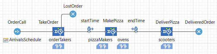
Notice that for measuring the cycle time of MakePizza activities, the corresponding processing node is included in a TimeMeasureStart-TimeMeasureEnd pair of time measurement nodes (startTime and endTime).
Unfortunately, PN modeling tools, like AnyLogic, do not support the general concept of activities (and Activity Networks), but only the special concept of processing activities. A processing activity has a processing object ("entity") as a mandatory participant, in addition to resource objects. While in a PN model, processing nodes do have a location and a processing capacity (the number of processing objects that can be processed in parallel), the nodes of an Activity Network (like the Make-and-Deliver-Pizza model), representing pure activities, in general do neither have a processing capacity nor a location.
For instance, in the AnyLogic Make-and-Deliver-Pizza model above, "orders" are processing objects and the processing activity TakeOrder is performed at the processing node TakeOrder by a pizza maker that is processing an "order". Consequently, the TakeOrder, MakePizza and DeliverPizza elements in the AnyLogic process diagram do not represent activities, but rather processing nodes.
Implementing the Enriched Process Design Model with AnyLogic
T.B.D.
10.1.3. Implementation with Simio
We want to implement the Make-and-Deliver-Pizza business process model model of Section 10.1 with Simio. For the reader's convenience, we show this model again in the following diagram:
For implementing the Make-and-Deliver-Pizza model with Simio, we use Simio's Facility view and its Standard Library where the PN modelling concept of an entry node is called "Source", a processing node is called "Server" and an exit node is called "Sink". We (1) first drag and drop a "Source" element from Simio's Standard Library and rename it to OrderCall, followed by (2) three "Server" elements, renamed to TakeOrder, MakePizza and DeliverPizza, followed by (3) a "Sink" element renamed to ReceivePizza.
In addition, we define:
- two individual Resource objects orderTaker1 and orderTaker2, which are placed in a Simio Object List orderTakers representing a resource pool for the TakeOrder activity;
- six individual Resource objects pizzaMaker1, ..., pizzaMaker6, which are placed in a Simio Object List pizzaMakers representing a resource pool for the MakePizza activity;
- two count pools ovens and scooters in the form of Simio Resource objects with capacities 3 and 10, respectively.
This results in the following Simio process diagram:
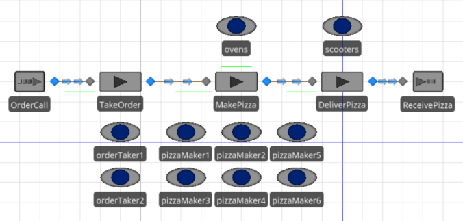
10.2. Load-Haul-Dump

A haul service company accepts requests for hauling large quantities of earth from a loading site to a dump site, using dump trucks and wheel loaders.
You can run this model from the Sim4edu website, or inspect its OESjs code.
Our Load-Haul-Dump modeling problem is based on the chapter "Example Model 2: Earthmoving operation" in the book The Art of Process-Centric Modeling with AnyLogic by Arash Mahdavi.
Conceptual Model
A haul service company has resource pools for dump trucks and wheel loaders. While the activities go (back) to loading site, haul, dump and go home just require a truck (or a wheel loader) as a resource, load activities require both a truck and a wheel loader.
Conceptual Information Model
The potentially relevant object types are:
- haul service company,
- wheel loaders,
- dump trucks.
Potentially relevant types of events and activities are:
- haul requests coming in from customers,
- going to the loading site (an activity performed by trucks and by wheel loaders),
- loading (performed by wheel loaders using trucks as resources),
- hauling (performed by trucks),
- dumping (performed by trucks),
- going back to loading site (performed by trucks),
- going home when the job is done (performed by trucks and by wheel loaders).
Both object types and event types, together with their participation associations, can be visually described in a conceptual information model in the form of a special kind of UML class diagram, called Object Event (OE) class diagram, as shown below.

Notice that the association end annotations «rr» and «rp» denote resource roles and resource pools. A haul service company has resource pools for trucks and wheel loaders. The activity types haul, dump and go back to loading site have a resource role truck for assigning a truck to any activity of one of those types. The activity types go to loading site and go home have either a a resource role truck or a resource role wheel loader, as indicated by the alternative association constraint expressed with a dashed line annotated with {xor}. The activity type load has both resource role truck and a resource role wheel loaders for assigning at least one and at most two wheel loaders to any load activity (as indicated by the multiplicity "1..2" at the «rr» association end at the class wheel loaders).
Conceptual Process Model
The involved types of events and activities can be related with each other via resource-dependent activity scheduling arrows and event scheduling arrows, as shown in the following DPMN process diagram:

Notice that there are three types of arrows in this DPMN diagram:
- Event Scheduling arrows, like the one between load and haul, have the meaning that the succeeding activity is started as soon as the preceding activity has been completed (there is no need for enqueuing a planned activity, since all resources required by the succeeding activity are provided by the preceding activity). Event Scheduling arrows are not part of BPMN, rather they have been proposed by Schruben (1983) for Event Graphs.
- A Multiple Events Scheduling arrow, like the one between requests and go to loading site, means that one instance of the preceding event type triggers multiple instances of the succeeding event type. In our example model, this means that one request event is followed by multiple go to loading site activities, one for each truck and each wheel loader assigned to the job.
- A Resource-Dependent Activity Scheduling arrow, like the one between go to loading site and load activities, means that as soon as an activity of the preceding activity type has been completed, a new planned activity is added to the queue of planned activities of the succeeding type (and started as soon as all required resources are available).
The model shows that when a haul request comes in, the haul service company deploys multiple trucks and wheel loaders to the loading site, each of them performing a go to loading site activity, as indicated by the double arrow between the haul requests event circle and the go to loading site activity rectangle. Each of these activities leads to enqueuing a new planned load activity, as indicated by the resource-dependent activity scheduling arrow from the go to loading site activity shape to the load activity shape. Such an enqueued (planned) activity is going to be dequeued and started as soon as the required resources become available. This means that as soon as a wheel loader is available, the next load activity is going to be started. When a load activity is completed, a haul activity and then a dump activity are going to start immediately, as indicated by the event scheduling arrows between them.
A more complete model prevents trucks to go back to the loading site and perform a load activity even when the job has been completed during the go back activity (resulting in haul and dump activities with an empty truck). For avoiding this uneconomic behavior, a second decision if the job has been done needs to be taken after the go back activity. In addition, the model has to describe that wheel loaders also go home when their job has been done. This is shown in the following refined model:

Simulation Design
In our simulation design, we consider only one particular haul service company, which does not have to be modeled as an explicit object. Also, we abstract away from the fact that also wheel loaders have to go to, and return from, the loading site by assuming that they are already at the site when the dump trucks arrive.
Information Design Model
In the information design model, we need to define a status attribute for all resource object types, such as Truck and WheelLoader, and a duration function, typically representing a random variable, for each activity type:

Notice how functions representing random
variables, like the duration function of all activity types,
are marked with the keyword (or UML 'stereotype') «rv» standing for "random
variable". These random variable functions sample from a probability
distribution function (PDF), which is symbolically indicated with
expressions like Tri(30,50,40) standing for the triangular PDF with lower
and upper bounds 30 and 50, and a median of 40.
Each activity type is associated with Truck or WheelLoader as their resource role(s), indicated with the association end stereotype «rr» standing for "resource role".
Process Design Model
A process design model, in the form of a DPMN process diagram as shown below, is derived from a conceptual process model by
- Abstracting away from items that are not design-relevant.
- Defining event variables, if needed.
- Defining object variables in the form of Data Object boxes for specifying state changes of objects affected by events.
- Formalizing decision conditions on the basis of event and object variables.

10.2.1. Implementation with OESjs
The JavaScript-based simulator OESjs implements the Object Event Simulation paradigm, and, consequently, allows a straight-forward coding of OE class models and DPMN process models.
Implementing the Information Design Model
For implementing the OE class design model with OESjs, we have to code all object types, event types and activity types specified in the model in the form of JavaScript classes.

The
Truck object class can be coded with OESjs-Core2 in the
following way:
class Truck extends oBJECT {
  constructor({ id, name, status}) {
    super( id, name);  // invoke the oBJECT constructor
    this.status = status;
  }
}
// a class-level attribute
Truck.capacity = 15;  // m3
All object classes inherit an
id attribute and a name attribute from the
pre-defined OES foundation class oBJECT. Since trucks are
resource objects, we need to define a status property for them.
We also define a class-level attribute capacity for modeling
their load capacity, assuming that all trucks have the same
capacity.
The WheelLoader object class is coded in the same way as Truck.

The
HaulRequest event class can be coded in the following
way:
class HaulRequest extends eVENT {
  constructor({ occTime, delay, quantity}) {
    super({occTime, delay});
    this.quantity = quantity;
  }
  onEvent() {
    ...
  }
}
All event classes inherit an occTime attribute and a
delay attribute from the pre-defined OES foundation class
eVENT. Any event in OES can be created either with a value for
the attribute occTime (standing for occurrence time)
or with a value for the attribute delay. In the latter case,
the event's occurrence time is automatically derived by adding the value of
delay to the current simulation time. In addition, the
HaulRequest event class has a property quantity for
specifying the quantity to be hauled.
The onEvent method
of the HaulRequest event class is not part of the information design
model. Rather, it is implementing an event rule specified in the process
design model. Consequently, it will be discussed below.

The GoToLoadingSite activity class can be coded in the following way:
class GoToLoadingSite extends aCTIVITY {
  constructor({id, startTime, duration}={}) {
    super({id, startTime, duration});
  }
  static duration() {return rand.triangular( 30, 50, 40);}
}
GoToLoadingSite.resourceRoles = {
  "truck": {range: Truck}
}
All activity classes inherit the attributes id,
startTime and duration from the pre-defined OES
foundation class aCTIVITY. When an activity is created as a JS
object during a simulation run, the value of its duration
property is obtained by invoking the duration() function
defined as a class-level ("static") function for its activity class. These
activity duration functions typically implement a random variable by
invoking a random variate sampling function, such as
rand.triangular(30,50,40), which samples from the triangular
probability distribution function (with min/max=30/50 and
mode=40).
Notice how the resource role association between
GoToLoadingSite and Truck, which defines the resource
reference property GoToLoadingSite::truck, is coded by a
corresponding entry in the map-valued class-level property
resourceRoles.
Implementing the Process Design Model
A
DPMN process design model can be decomposed into a set of event rule design
models, one for each type of event specified in the design model. Starting
with the HaulRequest event rule design model, we show how the
event rules specified by each of these event rule design models can be coded
in the form of an onEvent method.
HaulRequest event rule.
In the following HaulRequest event
rule method onEvent, all available trucks are allocated to the
current haul request, and, after computing the number of loads, for each of
the allocated trucks a new GoToLoadingSite activity is
started:
class HaulRequest extends eVENT {
  ...
  onEvent() {
    const followupEvents=[],
          allocatedTrucks = sim.resourcePools["trucks"].allocateAll();
    // assign model variable
    sim.model.v.nmrOfLoads = Math.ceil( this.quantity / Truck.capacity);
    for (const t of allocatedTrucks) {
      const goActy = new GoToLoadingSite();
      // assign truck as required resource
      goActy.truck = t;
      // start GoToLoadingSite activity
      followupEvents.push( new aCTIVITYsTART({plannedActivity: goActy}));
    }
    return followupEvents;
  }
}
Since activities are composite events, we also have event rules for them. The following GoToLoadingSite event rule is triggered whenever a GoToLoadingSite activity is completed, since the completion of an activity counts as its occurrence event.
GoToLoadingSite event rule.
This rule states that whenever a GoToLoadingSite activity ends (or is completed), then a new planned Load activity is enqueued, if no wheel loader is available, or, otherwise, a new Load activity is started. In OESjs, it is coded in the following declarative way:
GoToLoadingSite.successorActivity = "Load"
Such a successor activity assignment allows the simulator to check if the required resources are available and then start the successor activity, or, otherwise, enqueue a new planned successor activity.
Load
event rule.
This rule states that whenever a Load activity ends, the model variable nmrOfLoads is decremented by 1, and a Haul activity is immediately started (as a successor activity). Since the Haul activity doesn't require any additional resources, there is no need to enqueue a planned activity and wait for the availability of resources. In OESjs, this rule is coded in the following way:
class Load extends aCTIVITY {
  ...
  onActivityEnd() {
    // decrement nmrOfLoads counter
    sim.model.v.nmrOfLoads--;
    return [];  // no follow-up events
  }
  ...
}
Load.successorActivity = "Haul";
Notice that the state change
expressed in the modelVariables object rectangle, the decrementation
of nmrOfLoads, is taken care of in the onActivityEnd
method of the Load activity class. Instead of explicitly
scheduling the start of the succeeding Haul activity in that
method, we simply define Haul to be the successor activity of
Load.
Haul event rule.
The Haul event rule states that whenever a Haul activity ends, it is immediately succeeded by a Dump activity. It is coded in the following way:
Haul.successorActivity = "Dump";
Dump event rule.
The Dump event rule states that when a Dump activity ends and the model variable nmrOfLoads has the value 0, it is immediately succeeded by a GoHome activity, otherwise it is immediately succeeded by a GoBackToLoadingSite activity. The rule is coded by defining the successor activity as a function returning either "GoBackToLoadingSite" or "GoHome" in the following way:
Dump.successorActivity = function () {
  return sim.model.v.nmrOfLoads === 0 ? "GoHome":"GoBackToLoadingSite";
}GoBackToLoadingSite event rule.
The GoBackToLoadingSite event rule states that when a GoBackToLoadingSite activity ends and the model variable nmrOfLoads still has a value greater than 0, a new planned Load activity is enqueued; otherwise a GoHome activity is immediately started. The rule is coded by defining the successor activity of GoBackToLoadingSite as a function returning either "Load" or "GoHome" in the following way:
GoBackToLoadingSite.successorActivity = function () {
  return sim.model.v.nmrOfLoads > 0 ? "Load":"GoHome";
}10.2.2. Implementation with AnyLogic
Since AnyLogic does not support modeling plain activities (in Activity Networks), but only processing activities (in PNs with "entities flowing through the system"), it does not allow a straight-forward coding of the Load-Haul-Dump process design model (and its underlying class model). Rather, we have to figure out what we could use as "entities" for being able to make an AnyLogic PN model.
One option is to use the five trucks of the haul service company as the entities (called "agents" in AnyLogic), which arrive at a truck entry node and "flow" through the processing nodes Load, Haul and Dump before they leave the system via a truck exit node. Although this approach is quite artificial, imposing the PN paradigm on the given problem, it allows us using AnyLogic.
Notice that AnyLogic, like many other simulation tools, has adopted the Seize-Delay-Release pattern for modeling resource-constrained activities introduced by the simulation language GPSS in 1961. This means that activities are essentially modeled as Delay elements.
Implementing the Information Design Model with AnyLogic
From the information design model, we can only take the following items into consideration:
- All model variables are implemented as AnyLogic variables (defined in Main).
- The duration functions defined in activity types are implemented as the Delay times of corresponding AnyLogic Delay or Service elements.
- The resource roles defined for activity types are implemented either as Seize elements or as Seize information items within Service elements (if they had not to be transformed into entities, like the trucks of the Load-Haul-Dump model).
For instance, the activity type Load with its resource roles wheelLoader and truck, as defined in , is implemented as a Service element with
- its duration function, sampling the U(10,20) distribution, entered as "uniform(10,20)" in the Delay time field of the Load Service element.
- its resource role wheelLoader entered in the form of a resource pool wheelLoaders in the Resource pool field of the Load Service element, and its resource multiplicity constraint of exactly one entered as "1" in the field number of units.
Implementing the Process Design Model with AnyLogic
For facilitating a comparison between the DPMN process design model and the corresponding AnyLogic process model, we show the DPMN model again:

While the DPMN
process starts with the event HaulRequest, the AnyLogic process
starts with the entry node truckEntry (a "source" element) having the
field "Arrivals defined by" set to "Calls of inject() function",
which means that, for creating 5 trucks arriving at truckEntry, the
inject function needs to be invoked in the "On startup" procedure of
Main in the following way:
truckEntry.inject(5).
For simplicity, the activity nodes GoToLoadingSite and GoHome of the DPMN model are discarded.
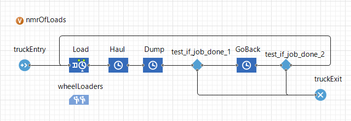
As explained above, the activity type Load is implemented as a Service element with a "Delay time" of "uniform(10,20)" and the field "Resource pool" set to "wheelLoaders" with "number of units" set to 1.
All other activity types are implemented as Delay elements (with a "Delay time" provided by their duration function defined in the class model).
The two decision diamonds of the DPMN model are implemented with corresponding "SelectOutput" elements called "test_if_job_done_1" and "test_if_job_done_2".
Unfortunately, PN modeling tools, like AnyLogic, do not support the general concept of activities (and Activity Networks), but only the special concept of processing activities. A processing activity has a processing object ("entity") as a mandatory participant, in addition to resource objects. While in a PN model, processing nodes do have a location and a processing capacity (the number of processing objects that can be processed in parallel), the nodes of an Activity Network (like the Load-Haul-Dump model), representing pure activities, in general do neither have a processing capacity nor a location.
For instance, in the AnyLogic Load-Haul-Dump model above, trucks are processing objects and the processing activity Load is performed at the processing node Load by a wheel loader that is processing a truck. Consequently, the Load, Haul, Dump and GoBack elements in the AnyLogic process diagram do not represent activities, but rather processing nodes.
10.2.3. Implementation with Simio
Since Simio, like AnyLogic, does not support modeling plain activities (in Activity Networks), but only processing activities (in PNs with "entities flowing through the system"), it does not allow a straight-forward coding of the Load-Haul-Dump process design model (and its underlying class model). Rather, we have to figure out what we could use as "entities" for being able to make a Simio PN model.
As before, we choose to use the five trucks of the haul service company as the "entities", which arrive at a truck entry node and "flow" through the processing nodes Load, Haul and Dump before they leave the system via a truck exit node. Although this approach is quite artificial, imposing the PN paradigm on the given problem, it allows us using Simio.
Notice that Simio, like many other simulation tools, has adopted the Seize-Delay-Release pattern for modeling resource-constrained activities introduced by the simulation language GPSS in 1961. This means that activities are essentially modeled as Delay elements.
Implementing the Information Design Model with Simio
From the information design model, we can only take the following items into consideration:
- All model variables are implemented as Simio variables (defined in Main).
- The duration functions defined in activity types are implemented as the Delay times of corresponding Simio Delay or Service elements.
- The resource roles defined for activity types are implemented either as Seize elements or as Seize information items within Service elements (if they had not to be transformed into entities, like the trucks of the Load-Haul-Dump model).
For instance, the activity type Load with its resource roles wheelLoader and truck, as defined in , is implemented as a Service element with
- its duration function, sampling the U(10,20) distribution, entered as "uniform(10,20)" in the Delay time field of the Load Service element.
- its resource role wheelLoader entered in the form of a resource pool wheelLoaders in the Resource pool field of the Load Service element, and its resource multiplicity constraint of exactly one entered as "1" in the field number of units.
Implementing the Process Design Model with Simio
For facilitating a comparison between the DPMN process design model and the corresponding Simio process model, we show the DPMN model again:
For implementing this process model as a Simio PN model, we need to model where the PN modelling concept of , a processing node is called "Server" and an exit node is called "Sink". We (1) first drag and drop a "Source" element from Simio's Standard Library and rename it to OrderCall, followed by (2) three "Server" elements, renamed to TakeOrder, MakePizza and DeliverPizza, followed by (3) a "Sink" element renamed to ReceivePizza.
- the HaulRequest event node as an entry node called "Source" in the Standard Library of Simio's Facility view;
- the activity nodes Load, Haul, Dump
While the DPMN process starts with the event HaulRequest,
the Simio process starts with the entry node truckEntry (a "source"
element) having the field "Arrivals defined by" set to "Calls of
inject() function", which means that, for creating 5 trucks arriving at
truckEntry, the inject function needs to be invoked in the "On
startup" procedure of Main in the following way:
truckEntry.inject(5).
In addition, we define:
- two individual Resource objects orderTaker1 and orderTaker2, which are placed in a Simio Object List orderTakers representing a resource pool for the TakeOrder activity;
- six individual Resource objects pizzaMaker1, ..., pizzaMaker6, which are placed in a Simio Object List pizzaMakers representing a resource pool for the MakePizza activity;
- two count pools ovens and scooters in the form of Simio Resource objects with capacities 3 and 10, respectively.
This results in the following Simio process diagram, where, for simplicity, the GoToLoadingSite activity of the DPMN model is discarded:
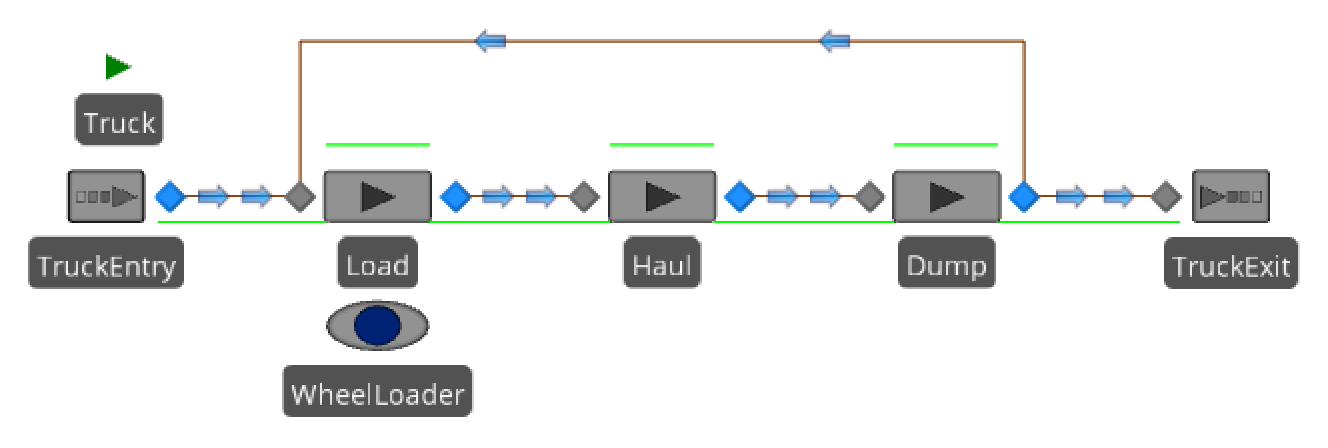
As explained above, the activity type Load is implemented as a Service element with a "Delay time" of "uniform(10,20)" and the field "Resource pool" set to "wheelLoaders" with "number of units" set to 1.
All other activity types are implemented as Delay elements (with a "Delay time" provided by their duration function defined in the class model).
The two decision diamonds of the DPMN model are implemented with corresponding "SelectOutput" elements called "test_if_job_done_1" and "test_if_job_done_2".
Unfortunately, PN modeling tools, like Simio and AnyLogic, do not support the general concept of activities (and Activity Networks), but only the special concept of processing activities. A processing activity has a processing object ("entity") as a mandatory participant, in addition to resource objects. While in a PN model, processing nodes do have a location and a processing capacity (the number of processing objects that can be processed in parallel), the nodes of an Activity Network (like the Load-Haul-Dump model), representing pure activities, in general do neither have a processing capacity nor a location.
For instance, in the Simio Load-Haul-Dump model above, trucks are processing objects and the processing activity Load is performed at the processing node Load by a wheel loader that is processing a truck. Consequently, the Load, Haul, Dump and GoBack elements in the Simio process diagram do not represent activities, but rather processing nodes.
Part IV. Processing Activities and Processing Networks
A Processing Activity is a resource-constrained activity that takes one or more objects as inputs and processes them in some way (possibly transforming them). The processed objects have been called "transactions" in GPSS, "entities" in SIMAN/Arena and also "jobs" in the Operations Research literature, while they are called processing objects in DPMN.
Ontologically, there are one or more objects participating in an activity, as shown in the diagram below. Some of them represent resources, while others represent processing objects. For instance, in the information and process models of a medical department shown in Figure 9-6 and Figure 9-9, there are two processing activity types: walks to room and examinations. In walks to room, since nurses are walking patients to examination rooms, nurses and rooms are resources, while patients are processing objects. In examinations, doctors and rooms are resources, while patients are processing objects. If patients would walk to an examination room by themselves (without the help of a nurse), patients would be the performers of walks to a room, and not processing objects, and, consequently, walks to a room would not be processing activities.

Processing activities typically require immobile physical resources, like rooms or workstation machines, which define the inner nodes of a Processing Network (PN). A Processing Object enters such a network via an Arrival event at an Entry Station, is subsequently routed along a chain of Processing Stations where it is subject to Processing Activities, and finally exits the network via a Departure event at an Exit Station.
The nodes of a PN define locations in a network space, which may be based on a two- or three-dimensional Euclidean space. Consequently, OEM-PN models are spatial simulation models, while basic OEM and OEM-A allow to abstract away from space. When processing objects are routed to a follow-up processing activity, they move to the location of the next processing node. The underlying space model allows visualizing a PN simulation in a natural way with processing objects as moving objects.
Each node in a PN model represents both an object and an event type. An Entry Node represents both an Entry Station (e.g., a reception area or an entrance to an inventory) and an arrival event type. A Processing Node represents both a Processing Station (e.g., a workstation or a room) and a processing activity type. An Exit Node represents both an Exit Processing and a departure event type.
A Processing Flow arrow connecting a Processing Node with another Processing Node or with an Exit Node represents both an event flow and an object flow. Thus, the node types and the flow arrows of a PN are high-level modeling concepts that are overloaded with two meanings.
A PN modeling language should have elements for modeling each of the three types of nodes. Consequently, DPMN-A has to be extended by adding new visual modeling elements for entry, processing and exit nodes, and for connecting them.
In the field of DES, PNs have often been characterized by the narrative of “entities flowing through a system”. In fact, while in basic DPMN and in DPMN-A, there is only a flow of events, in DPMN-PN this flow of events is over-laid with a flow of (processing) objects.
PNs have been investigated in operations management and the mathematical theory of queuing (Loch 1998, Williams 2016) and have been the application focus of most industrial simulation software products, historically starting with GPSS (Gordon 1961) and SIMAN/Arena (Pegden and Davis 1992). They allow modeling many forms of discrete processing processes as can be found, for instance, in the manufacturing industry and the services industry.
It is remarkable that the PN paradigm has dominated the discrete event simulation market since the 1990’s and still flourishes today, mainly in the manufacturing and services industries, often with object-oriented and “agent-based” extensions. Its dominance has led many simulation experts to view it as a synonym of DES, which is a conceptual flaw because the concept of DES, even if not precisely defined, is clearly more general than the PN paradigm.
The PN paradigm has often been called a “process-oriented” DES approach. But unlike the business process modeling language BPMN, it is not concerned with a general concept of business process models, but rather with the special class of processing process models for discrete processing systems. A processing process includes the simultaneous handling of several “cases” (processing objects) that may compete for resources or have other interdependencies, while a “business process” in Business Process Management has traditionally been considered as a case-based process that is isolated from other cases.
For PN models, a simulator can automatically collect the following statistics, in addition to the resource-constrained activities statistics described in 9. Resource-Constrained Activities:
- The number of processing objects that arrived at, and departed from, the system.
- The number of processing objects in process (that is, either waiting in a queue/buffer or being processed)
- The average time a processing object spends in the system (also called throughput time).
During a simulation run, it must hold that the number of processing objects that arrived at the system is equal to the sum of the number of processing objects in process and the number of processing objects that departed from the system, symbolically:
Chapter 11. Conceptual Modeling of Processing Networks
For accommodating PN modeling, OEM-A is extended by adding pre-defined types for processing objects, entry node objects, arrival events, processing node objects, processing activities, exit objects and departure events, resulting in OEM-PN. These "built-in" types, which are described in Figure 11-1, allow making PN models based on them simply by making a process model (with DPMN) without the need of making an information/class model as its foundation, as shown in Figure 11-2.

An example of a conceptual PN model: Department of Motor Vehicles
As a simple example of a PN simulation model we consider a Department of Motor Vehicles (DMV) with two consecutive service desks: a reception desk and a case handling desk. When a customer arrives at the DMV, she first has to queue up at the reception desk where data for her case is recorded. The customer then goes to the waiting area and waits for being called by the case handling desk where her case will be processed. After completing the case handling, the customer leaves the DMV via the exit.
Customer arrivals are modeled with an «entry node» element (with name “DMV entry”), the two consecutive service desks are modeled with two «processing node» elements, and the departure of customers is modeled with an «exit node» element (with name “DMV exit”).
DPMN is extended by adding the new modeling elements of
- Entry/Processing/Exit Node rectangles representing node objects that take the form of stereotyped UML object rectangles;
- Processing Flow arrows representing the combination of an object flow arrow with an RDAS arrow (pointing to processing nodes), having a special arrow head consisting of a circle and three bars, as shown in Figure 11-2;
- Object-Event Flow arrows, representing the combined object-event flow from processing nodes to exit nodes, as shown in Figure 11-2.

Using both Processing Flow arrows and Event Flow arrows
While a Processing Flow arrow between two nodes implies both a flow of the processing object to the successor node and the resource-dependent scheduling of the next processing activity, an Event Flow arrow from a processing node to an Event circle represents an event flow where a processing activity end event causes/schedules another event, as illustrated in the example of Figure 11-3.

Chapter 12. Processing Network Design Models
For accommodating PN modeling, OEM-A is extended by adding pre-defined types for processing objects, entry node objects, arrival events, processing node objects, processing activities, exit objects and departure events, resulting in OEM-PN. These "built-in" types, as described in Figure 12-1, allow making PN models based on them simply by making a process model with DPMN without the need of making an OEM class model as its foundation, as shown in Figure 12-2.

Notice that the range of the properties arrivalRecurrence, successorNodes and
duration of the built-in object types EntryNode and ProcessingNode is Function, which means that the value of such
a property for a specific node is a specific function. While the standard UML semantics does not support such an extension of the semantics of
properties in the spirit of the Functional Programming paradigm, its implementation in a functional OO programming language like
JavaScript, where objects can have instance-level functions/methods, is straightforward.
The property successorNodes allows to express a function that provides, for any given entry or processing node, a (possibly singleton) set of processing nodes or exit nodes. Such a function can express several cases of routing a processing object from a node to one or more successor nodes:
- a fixed unique successor node for modeling a series of processing nodes connected by (possibly conditional) object flow arrows, as in Figure 12-4;
- a conditional unique successor node for modeling an Exclusive (XOR) Gateway leading to one of several possible successor nodes;
- a variable subset of a set of potential successor nodes for modeling an Inclusive (OR) Gateway;
- a fixed set of successor nodes for modeling a Parallel (AND) Gateway;
In a DPMN diagram, the set of successor nodes of a node is defined by Flow Arrows, possibly in combination with Gateways.
PN example 1: a single workstation
Part arrivals are modeled with an «entry node» element (with name “partEntry”), the workstation is modeled with a «processing node» element, and the departure of parts is modeled with an «exit node» element (with name “partExit”).
DPMN is extended by adding the new modeling elements of PN Node rectangles, representing node objects with associated event types, and PN Flow arrows, representing combined object-event flows. PN Node rectangles take the form of stereotyped UML object rectangles, while PN Flow arrows have a special arrow head, as shown in Figure 12-2.

PN example 2: a workstation may have to rework parts
Parts that turn out to be defective after being processed need to be reworked. This can be modeled by adding an attribute percentDefective to the object type Workstation and suitable logic to the Processing activity end event rule such that in percentDefective % of all cases a processed part cannot depart the system (i.e., is not removed from the input buffer), but is being reworked by another Processing activity.

PN example 3: Department of Motor Vehicles
A Department of Motor Vehicles (DMV) has two consecutive service desks: a reception desk and a case handling desk. When a customer arrives at the DMV, she first has to queue up at the reception desk where data for her case is recorded. The customer then goes to the waiting area and waits for being called by the case handling desk where her case will be processed. After completing the case handling, the customer leaves the DMV via the exit.
Customer arrivals are modeled with an «entry node» element (with name “dmvEntry”), the two consecutive service desks are modeled with two «processing node» elements, and the departure of customers is modeled with an «exit node» element (with name “dmvExit”).

Chapter 13. Case Studies
13.1. Diagnostic Department


At a diagnostic department of a hospital, incoming patients first get recordings of their heart’s electrical activity via an Electrocardiography (ECG) and then get an ultrasound scan.
For getting a quick impression, you can run this model from the Sim4edu website, or inspect its OESjs code.
Our Diagnostic Department modeling problem is based on the chapter "Example Model 4: Clinic" in the book The Art of Process-Centric Modeling with AnyLogic by Arash Mahdavi.
The diagnostic process consists of two subprocesses:
Performing the ECG: When a patient enters the clinic, they must wait in a waiting area for their name to be called. A patient whose name is called will walk to the “ECG room”, choose a free spot and wait for an ECG technician. ECG technicians have to walk from the “ECG technician room” to the “ECG Room” after being requested to a new patient. They will first go to the “ECG storage room", pick up an ECG machine, bring it to the waiting patient in the ECG room and start the ECG procedure. When the ECG procedure is completed, the technician returns the ECG machine to the storage room and walks back to the ECG technician room. After each procedure, ECG technicians rest for five minutes before they accept a new patient. A patient who has completed the ECG will not leave the ECG room until there is an available spot in the “ultrasound room”.
Performing the ultrasound (US) scan: At the start of this procedure, a patient is done with the ECG but still waiting in the ECG room for a free spot in the US room. Each US spot is a combination of a US machine and the bed it's assigned to. When there is an available spot, the patient's name is called; they walk to the assigned bed and lay down on it. At this point, the patient is ready and a request for a doctor is sent to the “Doctors on Call” room. If there is no doctor available (that is, they are resting or with other patients), the patient must wait until a doctor becomes available. When an on‐call doctor is readily available, they will walk to the patient's bed in the US room and start the US scan.
The department's management has the following business objectives:
- Process 50 patients during each operating day.
- Minimize the time to process patients (also called throughput time), as this is the most important indicator of patient satisfaction.
- Complete the ECG and US procedures for all admitted patients by the end of the department's daily working hours (within eight hours) and without the need for after-hour work.
The purpose of this modeling and simulation project is to find system designs that fulfill the above business objectives. For observing if a system design fulfills the objectives, we can use the following simulation statistics: (a) average throughput time, (b) utilization of resources, (c) the departure time of the last patient (used as a measure of daily operation duration)
Conceptual Model
The diagnostic department under consideration has resource pools for ECG spots, ECG technicians, ECG machines, US beds, US machines and doctors. While a perform ECG activity is performed by an ECG technician using an ECG machine and an ECG spot, a perform US activity requires a doctor using a US machine and a US bed.
For simplicity, we make a non-spatial (purely temporal) model, not modeling any spatial aspects, as opposed to the model discussed in The Art of Process-Centric Modeling with AnyLogic.
Conceptual Information Model
The potentially relevant object types are:
- diagnostic departments (the organizational units that own/manage their diagnosis business processes);
- patients;
- the seven spaces/rooms: waiting area, ECG room, ECG technician room, ECG storage room, ultrasound room, "doctors on call" room, doctors resting room;
- the six resource object types ECG spots, ECG technicians, ECG machines, US beds, US machines and doctors.
Potentially relevant types of events and activities are:
- arrivals of new patients;
- patients walking to the ECG room;
- ECG technicians (a) walking to the ECG storage room, (b) moving an ECG machine from the ECG storage room to the ECG room, (c) performing an ECG on a patient, (d) returning the ECG machine to the storage room, (e) walking back to the ECG technician room, and (f) resting for five minutes;
- patients going from the ECG room to the US room,
- doctors (a) walking from the "doctors on call" room to the patient's bed in the US room, (b) performing an US scan on the patient, (c) walking to the doctors resting room, (d) resting for some time, and (e) going back to the "doctors on call" room;
- departure of patients.
When making a process model, we normally adopt the perspective of the organization (or organizational unit) that "owns" the business process to be modeled, here: the diagnostic department. Notice the conceptual issue that the activities performed by patients (walking to the ECG room, going to the US room) are not ordinary business activities, since they are not performed by an organizational actor, such as a technician or doctor, counting as a resource. In their case, the performer (a patient) is not a resource. For this reason they will be modeled without a performer role.
Object, event and activity types, together with their participation associations, can be visually described in a conceptual information model in the form of a conceptual Object Event (OE) class diagram. The following OE class model describes the core elements of our diagnostic department viewed as a business system.

While this model defines primary business activity types together with their resource roles (association ends annotated with «rr»), associated resource types and corresponding resource pools (association ends annotated with «rp»), it does not capture the types of secondary business activities of
- ECG technicians (a) walking to the ECG storage room, (b) moving an ECG machine from that storage room to the ECG room, (c) returning the ECG machine to the storage room, (d) walking back to the ECG technician room, and (e) resting for five minutes;
- doctors (a) walking from the "doctors on call" room to the patient's bed in the US room, (b) walking to the doctors resting room, (c) resting for some time, and (d) going back to the "doctors on call" room.
These secondary business activities are described in the following OE class diagrams.


Conceptual Process Model
As service processes, health care processes can be viewed/modeled as Processing Networks (PNs). Since PNs are more high-level than Activity Networks (ANs), it is preferable to model the Diagnostic Department as a PN.
The following BPMN process diagram shows a coarse-grained conceptual process model of the primary business activities of the Diagnostic Department, with two swimlanes for the two performers of the process:

Unfortunately, as an AN modeling language, BPMN does not provide any special elements for modeling PNs. While BPMN allows modeling the performers of activities with lanes, it does not support modeling other types of resource objects. As a workaround, we have included the resource objects ECG spot, ECG machine and US bed in the form of BPMN Data Objects. But this does not allow to clearly display the processing nodes of a processing network as a combination of a processing station (like ECG spot) with its processing activity (like perform ECG).
An even more severe issue of the BPMN model is its uniform (semantically overloaded) use of "sequence flow" arrows for representing different types of flows: event flows, activity flows and processing flows. While in the case of an activity, incoming arrows do not mean that an activity is started, but rather that a new planned activity (or task) is enqueued and only started when all required resources become available, in the case of a processing node, an incoming arrow represents a processing flow, which is a combined object-event flow of processing objects and their delayed processing activity start events.
These issues of BPMN have been solved in DPMN, which supports the visual modeling of processing networks with processing nodes connected by processing flow arrows, as shown in the following DPMN process diagram:

This conceptual DPMN process diagram is based on the underlying OE class model discussed in the previous section. Notice that a two-part name of a processing node (like "ECG spot / perform ECG") contains both the name of the node's processing station ("ECG spot") and the name of the node's processing activity ("perform ECG"). For the processing node "ECG spot / perform ECG", the model specifies three resource objects: an "ECG technician" as the performer, the processing station "ECG spot" (specified in the node name), and an additional resource object "ECG machine".
Run this model from the OESjs GitHub website
While this model attains a highly compact description of the Diagnostic Department system by compressing "ECG spot" resources and the "perform ECG" activity, as well as "US bed" resources and the "perform US scan" activity, into a corresponding processing node, it abstracts away from the activities of patients walking to the ECG room and walking from the ECG room to the US room.
The above model can be further refined by explicitly modeling the two patient activities "walk to ECG spot" and "walk to US bed". While the first of them requires an "ECG spot" as a resource, the second one requires a "US bed". In the following DPMN process diagram, we do not display the rectangular container (called Pool) for the Diagnostic Department, leaving it implicit.

Notice that in this refined model, the processing nodes of the previous model have been resolved into corresponding processing activities (and associated resources).
According to DPMN's declarative resource modeling principles, a required resource will be allocated before an activity starts and, unless the follow-up activity also requires a resource of that type, released after it has completed. In the case of the activity sequence of "perform ECG" and "walk patient to US bed", however, the resource "ECG spot" must not be released before the follow-up activity "walk patient to US bed" starts, because it represents the location of the patient (in the ECG room), which only becomes available when the patient leaves the room (for going to the US room) and not when the "perform ECG" activity ends.
DPMN allows to mark such a deferred resource de-allocation with the help of a special resource role association end (a dot with a bar), as can be seen in the diagram at the "ECG spot" resource type rectangle. It means that this resource is not released when the activity (here "perform ECG") ends, but only when the follow-up activity (here "walk patient to US bed") starts.
In this example, the requirement for deferred resource de-allocation stems from the ambiguity of the ECG room (with three spots) representing both a spatial resource for the activity "perform ECG" and an input buffer for the processing activity "walk to US bed". This points to an intricate relationship between the concepts of spatial resources and input buffers in PNs, which requires further research.
Simulation Design
T.B.D.
Based on the two conceptual models discussed in the previous section, we are going to make two design models, a simpler (more abstract) one and a more detailed one. In both designs, we consider only one diagnostic department, which does not have to be modeled as an explicit object.
These secondary business activities will only be modeled in a third version of the Diagnostic Department model.
Diagnostic-Department-1
| Activity | Duration |
|---|---|
| perform ECG | |
We consider a scenario with two order takers, ten pizza makers, five ovens and 20 scooters.
Information Design Model
T.B.D.
An information design model, in the form of an OE class diagram as shown below, is derived from a conceptual information model by abstracting away from items that are not design-relevant and possibly adding certain computational details.
An OE class design diagram like the one above, defines resource roles, resource role types and resource multiplicity constraints for all types of activities. Normally, in an OE simulation there is a one-to-one correspondence between resource role types and resource pools. By convention, a resource pool has the same name as the corresponding resource role type, yet pluralized and starting with a lowercase character.
Process Design Model
T.B.D.
A process design model, in the form of a DPMN process diagram as shown below, is derived from a conceptual process model by abstracting away from items that are not design-relevant and possibly adding certain computational details.
A DPMN process design model essentially defines the admissible sequences of events and activities together with their dependencies and effects on objects, while its underlying OE class design model defines the types of objects, events and activities, together with the participation of objects in events and activities, including the resource roles of activities, as well as resource multiplicity constraints, parallel participation constraints, alternative resources, and task priorities.
It is an option, though, to enrich a DPMN process design model by displaying more computational details, especially the recurrence of exogenous events, the duration of activities and the most important resource management features defined in the underlying OE class design model, such as resource roles (in particular, performer roles can be displayed in the form of Lanes) and resource multiplicity constraints. The following model shows an enriched version of :
Such an enriched DPMN process design model includes all computational details needed for an implementation without a separate explicit OE class design model. In fact, such a process model implicitly defines a corresponding class model. For instance, the enriched DPMN model of implicitly defines the OE class model of above.
The notation for defining performer roles in Lanes consists of a performer role name (such as pizzaMakers) and and an object type name (such as PizzaMaker) denoting its range, separated by a colon. When the performer role name is appended by a multiplicity expression in brackets, as in pizzaMakers[2], this denotes a resource multiplicity constraint (stating that exactly 2 pizzaMakers are required). When only a performer type prefixed with a colon (such as :OrderTaker) is provided, this means that the implicit performer role name is obtained by lowercasing the performer type name (as in orderTaker:OrderTaker).
The notation for defining a non-performer resource role, such as oven:Oven, consists of a named object rectangle, such as the :Oven rectangle in , attached to an activity rectangle by means of a connection line with a small filled square representing a resource link, such as the line between the MakePizza activity rectangle and the :Oven object rectangle in .Notice that the model of does not include any element representing a resource pool. It is assumed that for any organizational position described in the underlying OE class model, the organization under consideration has a corresponding resource pool. By default , each resource role of an activity type is associated with a resource pool having the same (yet pluralized) name, such that its resources are instances of a corresponding resource role type, which is an organizational position in the case of human resources.
Combined with its underlying OE class design model, a DPMN process design model provides a computationally complete specification of a simulation model.
13.1.1. Implementation with OESjs
The JavaScript-based simulator OESjs-Core3 implements the Object Event Simulation (OES) Processing Networks paradigm, and, consequently, allows a straight-forward coding of OE class design models and DPMN process design models of Processing Networks.
Implementing the OE Class Design
Model
T.B.D.
13.1.2. Implementation with Simio
T.B.D.
13.1.3. Implementation with AnyLogic
T.B.D.
Part V. Agent-Based Modeling and Simulation
The term "agent-based modeling" is an umbrella term that subsumes many different approaches to simulation, typically focused on modeling (collections of) entities/objects/individuals/"agents" and their interactions with each other and with their environment. In any case, since the interactions of agents are based on discrete perception and action events, it is natural to define an agent-based modeling and simulation approach as an extension of a DES approach, such that it is an option to use the concept of agents along with the more basic concepts of objects and events. Along these lines, OEM&S can be extended by adding the concept of agents, together with concepts of perception and action events as well as communication, resulting in Agent/Object Event Modeling and Simulation (A/OEM&S).
In academic research, the term "agent-based" M&S is used ambiguously both for individual-based and cognitive agent M&S. The former, which is also called "microscopic" simulation (or micro-simulation), is focused on modeling (collections of) individuals and their interactions with each other and with their environment for modeling complex systems, whereas the latter is more concerned with modeling the cognitive state and cognitive operations of an agent.
Consequently, it seems natural to distinguish between a weak concept of agents, which we call basic agents, where agents are entities that interact with their environment and with each other, and a strong concept, called cognitive agents, that is based on modeling the cognitive (or mental) state and operations of agents.
The cognitive state of basic agents has only one component: their information state containing propositional information about their environment and about themselves resulting both from perception and from communication. A propositional information item of an information state can be expressed in the form of a triple statement (or, simply, triple), which is an atomic predicate logic sentence that consists of (1) an object name, (2) a property name, and (3) a property value. Such an information item can be viewed as a belief of an agent, or as a knowledge item (where knowledge means correct information or true belief).
Beliefs represent the typically partial and sometimes incorrect subjective information of agents about their environment and about themselves. They are the most basic component of the cognitive state of an agent. The simplest model of a cognitive state only consists of beliefs, while more advanced models may also include commitments, goals, intentions, emotions, etc.
Many agent-based (in particular, individual-based) M&S approaches do not attempt to support the incompleteness of beliefs/information or the possibility of incorrect beliefs/information. They make the (tacit) assumption that agents have perfect information and focus on modeling interactive behavior: (1) the interaction of an agent with its inanimate environment via a perception-action cycle, and (2) the communication between agents.
A general model of the interactive behavior of agents depends, at least, on their information state, which is
- queried for decision making, and from which information items are retrieved for informing other agents;
- updated when new information is obtained by means of perception or communication.
In the general case of a cognitive agent with possibly false beliefs, its belief state (or subjective information state) has to be represented as a kind of restricted and modified duplicate of the objective information state managed by the simulator, requiring a more complex simulator architecture. Within such an architecture, the information state of a perfect information agent has to be short-circuited with the objective information state managed by the simulator.
Chapter 14. Basic Agents with Perfect Information
Basic agents are objects that (1) have an information state, (2) may have perceptions of their environment affecting their information state, and (3) may communicate with each other and, as a consequence, change their information state. We define perfect information agents as basic agents that
- have complete and correct information about all objects they know;
- are sincere: they do not provide intentionally incorrect information in their communications with other agents (that is, they do not lie).
Condition 1 does not hold for physical agents in the real-world, such as humans, animals or robots. Rather it's a simplifying assumption that we may want to make in a simulation model abstracting away from the limitations of real-world agents. Condition 2 typically holds for robots (and other artifact agents), but not for humans.
In A/OEM&S, agents are, by default, perfect information agents with
two collection-valued properties, objects and agents, which represent their information state: the (non-agentive) objects and the agents they know;
two generic "event-handling" operations that are invoked by the simulator when processing perception events or message events:
- onReceive for handling in-message events (i.e., for receiving messages),
- onPerceive for handling perception events (i.e., for processing perceptions), and
two generic operations for performing actions and sending messages:
- perform for performing an action (by scheduling an action event),
- send for sending a message to one or more other agents (by scheduling a message event with one or more receivers).
Notice that actions are events and we therefore also call them action events. Sending a message corresponds to a send message action (also called an out-message action event).
These operations are depicted in the following diagram showing an A/OEM&S meta-model fragment:

In A/OEM&S, the behavior of an agent is based on in its event handling operations onPerceive and onReceive for reacting to perceptions and to incoming messages, as well as perform and send for performing actions and sending messages.
In a standalone (non-distributed) simulator for A/OEM&S, the most efficient way of implementing inter-agent communication is achieved by having the sender directly invoking a message reception method of the receiver (corresponding to synchronous message passing).
However, such an implementation (by direct method invocation) would bypass the fundamental event scheduling mechanism of OEM&S, which also warrants the occurrence time consistency of events. Each perception event and each action should be scheduled as an event, i.e., added to the simulator's Future Events List (FEL), such that it can be processed by the simulator on its occurrence time.
When the simulator processes a perception event as an objective (external) event from the FEL, it invokes the onPerceive event-handling method of the perceiver agent, which corresponds to a subjective (internal) perception event that is induced by the objective perception event.
In A/OEM&S, performing a send message action corresponds to scheduling a message event with a message, a sender and a receiver. When the simulator processes a message event as an objective (external) event from the FEL, it invokes the onReceive event-handling method of the receiver agent, which corresponds to a subjective (internal) message reception event that is induced by the objective message event.
There are two alternative architectures for simulating agents and their interactions with their environment and with each other:
- An interleaved architecture (based on next-event time progression) that interleaves the processing of events and the execution of agent behavior.
- A round-based architecture (based on incremental time progression) that, in a loop, transmits to each agent all perception and message events that affect it, and then waits for the resulting state changes and action events created by each agent, before it proceeds with first processing the state changes and then processing the next events. This approach guarantees that the behavior (and state changes) of an agent at each simulation step is not affected by the behavior (and state changes) of other agents at the same simulation step, but only by their past behavior (and state changes).
The interleaved architecture, allowing the immediate processing of perception events and message events by the simulator, is simpler and more efficient..
14.1. Perception and Action
Agents may perceive objects and events in their environment and, in response, take certain actions, possibly causing changes in their environment.
One can distinguish between a passive and an active form of perception. Passive perception takes place asynchronously, while an agent is busy or idle, in the form of (instantaneous) perception events, while active perception requires the agent to perform a perceptive action or activity (like scanning the neighborhood). In general, agents are exposed to perception events and may react in response to them.
In the case of physical agents, like robots, passive perception events are created by a sensor containing an event detector, such as a Proximity Infra-Red (PIR) sensor, which has its output pin going high whenever it detects an infra-red emitting object (e.g., a human or a medium to large sized animal) in its reach. Active perceptions are created by querying the measurement value of a sensor containing a quality detector, such as a DHT22 temperature and humidity sensor. The distinction between event detectors and quality detectors has been proposed in (Diaconescu and Wagner 2015).
Perception events typically lead to an update of existing beliefs or to the creation of new beliefs.
14.2. Communication
There are various forms of communication between agents. In particular, we can distinguish between verbal and non-verbal communication. We are only concerned with verbal communication, which is based on messages.
Ontological Considerations
Conceptually, a communication event is composed of two successive atomic events: an out-message event (corresponding to a send message action of the sender) and a correlated in-message event (or message reception by the receiver). This is illustrated by the following diagram:

This concept diagram expresses the following ontological stipulations:
A message is sent from a sender agent to one or more receiver agents via an out-message event.
A message from a sender agent is received by a receiver agent via an in-message event.
A communication event consists of a pair of correlated out/in message events out and in, such that the following conditions hold:
- in.message = out.message
- in.receiver is included in out.receivers
- in.sender = out.sender
- in.occurrenceTime > out.occurrenceTime
Communication events may lead to updates (and deletions) of existing beliefs or to the creation of new beliefs, especially in information exchange processes based on Tell-Ask-Reply messages.
Message Types
Each message is of a certain type defining its properties and implicit semantics. There are two kinds of message types:
- User-defined problem/domain-specific message types: the structure of such a message type is defined within a simulation model in the form of a class defining its properties; their semantics is defined in the receive methods of receiver agents in terms of how messages of such a type are processed.
- Pre-defined problem/domain-independent message types: Tell and Ask/Reply are examples of problem/domain-independent message types that may be supported by a simulator. As they refer to general speech acts, the semantics of these message types should be based on the philosophical speech act theory of Austin and Searle.

There are two prominent agent communication language standards: FIPA and KQML (Finin et al 1997), both defining domain-independent standard message types with a semantics based on speech act theory. We briefly describe the rules for processing Tell, Ask, Reply and Request messages:
- Tell
Using this message type, agents may communicate some of their beliefs to other agents, without being asked. In general, a teller may tell the truth or may lie; and in both cases the provided information may or may not be correct.
A Tell message is similar to what is called a Signal in the Unified Modeling Language (UML) where a Signal is sent asynchronously from an object to another object. The event rule for processing a Signal reception event is defined by specifying a Reception operation in the classifier of the receiver object, such that this operation has the same name as the type of the Signal (and a corresponding signature). We do not use these UML concepts (and the UML terminology) since they are too limited.
- Ask
- Using this message type, an agent may query another agent about some of its beliefs. Queries are expressed in a suitable query language, such as the RDF-based query language SPARQL. An asker expects to receive an answer via a Reply message some time later.
- Reply
- This message type is used for replying to a previously received Ask message. In general, the answers provided may or may not be correct. Therefore, askers should only update their beliefs according to the received answers when they trust the replier.
- Request
- This message type is used by an agent for requesting another agent to perform a certain action. Such a request can be either accepted or rejected.
Since a perfect information agent already has complete information about the objects it knows,
- sending a query via an Ask message only makes sense if the query may retrieve objects the sender does not yet know;
- sending an answer via a Reply message only makes sense if the answer provides information about objects the receiver does not yet know;
- receiving a statement via a Tell message only makes sense if the statement provides information about an object the receiver does not yet know.
14.3. Interleaved Agent Simulation
In interleaved agent simulation, the simulator processes a PerceptionEvent by invoking the method onPerceive of the perceiver agent. An agent performs an action, e.g., in response to a perception, with the help of its perform method, which schedules a corresponding ActionEvent that is then processed by the simulator.
Likewise, message-based communication is implemented by having the sender agent invoking its send method, which schedules a MessageEvent that is then processed by the simulator by invoking the onReceive method of the receiver agent. In this way, a MessageEvent is inserted into the simulation log and it is guaranteed that, as required above, the time when a message is received is later than the time it has been sent (in.occurrenceTime > out.occurrenceTime).
Perception and Action
For supporting perception events and actions, the OEM&S concept Event is extended in the following way:

This means that
- The pre-defined (abstract) object type Agent has two abstract
methods for perception and action:
- onPerceive to be invoked with a perception argument, which is a PerceptionEvent,
- perform to be invoked with an action argument, which is an Action.
- There are two pre-defined (abstract) event types: PerceptionEvent and Action.
- A PerceptionEvent has a perceiver reference and may have additional attribute values.
- When a PerceptionEvent is processed by the simulator, it invokes the onPerceive method of the perceiver agent and passes the perception (event). This implies that the code for realizing the effects of a perception event is included in the agent class (in its definition of the onPerceive method).
- An Action event has a performer reference and may have additional attribute values.
- When an agent performs an action by invoking the perform method, an Action event is scheduled, which is then processed by the simulator by invoking the onEvent method defined in the action event class. This implies that the code for realizing the effects of an action is included in the action event class (in its definition of the action event handler onEvent).
Message-Based Communication
The following diagram shows the new A/OEM&S elements added to the OEM&S meta-model:

This means that
- The pre-defined (abstract) class Agent has the abstract method onReceive to be invoked with a message and a sender reference.
- There is a pre-defined event type MessageEvent.
- A MessageEvent has a message attribute value, which is a string or a composite value.
- When a MessageEvent occurs, the simulator invokes the onReceive method of the receiver agent and passes the message attribute value. This implies that the code for realizing the effects of an in-message event is included in the agent class (in its definition of the onReceive method).
In a distributed simulator for A/OEM&S, where all agents of a simulation scenario run as different processes (on different computers) without a shared simulator state, and, consequently, message passing would be asynchronous, it would be natural to implement both out-message events and in-message events, as described above.
Agent-Based Simulation with OESjs
Typically, a sender agent sends a message (or schedules a MessageEvent) within its onPerceive or onReceive methods, that is, in response to a perception or to a message reception. In OESjs-Core4, this could be programmed in the following way:
1 2 3 4 5 6 7 8 9 10 11 12 13 14 15 16 17 18 | class Doctor extends aGENT {
constructor({ id, name, status}) {
super( id, name);
this.status = status;
}
onReceive( msg, sender) {
switch (msg.type) {
case "ASK":
const answer = this.processQuery( msg.query),
reply = new rEPLY( answer),
receiver = sender;
this.send( reply, receiver));
break;
case "REPLY":
...
}
}
} |
Often, a PerceptionEvent is scheduled as a consequence of an action event with the meaning that the action is perceived by another agent. A PerceptionEvent is processed by the simulator by invoking the onPerceive method of the perceiver agent while passing the perception attribute value.
An Action is typically performed by an agent within its onPerceive or onReceive methods in response to a perception or to a message reception. In OESjs, this could be programmed in the following way:
1 2 3 4 5 6 7 8 9 10 11 12 13 | class Doctor extends aGENT {
constructor({ id, name, status}) {
super( id, name);
this.status = status;
}
onPerceive( perceptionEvt) {
switch (perceptionEvt.constructor.name) {
case "CovidSymptom":
this.perform( new aCTION("performPCR"));
break;
}
}
} |
14.3.1. Case Study: A Four Stage Supply Chain
A four stage supply chain consists of a retailer, a wholesaler, a distributor and a factory. While the factory is a top SC node, which only receives orders from and ships the ordered items to its downstream node, all others also receive deliveries from and send orders to their upstream nodes.
For getting a quick impression, you can run this model from the Sim4edu website, or inspect its OESjs code.
Conceptual Model
Conceptual Information Model
The potentially relevant object types are:
- top supply chain nodes (like the factory),
- intermediate supply chain nodes (like the wholesaler and distributor),
- bottom supply chain nodes (like the retailer).
Potentially relevant types of events and activities are:
- receive order (from the downstream node or from end customer),
- end of week,
- send order (to the upstream node),
- ship items (to the downstream node),
- perceive reception of items (receive delivery).
Object, event and activity types, together with their participation associations, can be visually described in a conceptual information model in the form of a conceptual Object Event (OE) class diagram.

Conceptual Process Model

Simulation Design
Each SC node is modeled as an agent that reacts to
- the in-message event "receive order",
- the perception event "perceive reception of items" (delivery), and
- the time event "end of week",
and performs
- the out-message action "send order" and
- the action "ship items".
Information Design Model
T.B.D.
An information design model, in the form of an OE class diagram as shown below, is derived from a conceptual information model by abstracting away from items that are not design-relevant and possibly adding certain computational details.
Process Design Model
T.B.D.
A process design model, in the form of a DPMN process diagram as shown below, is derived from a conceptual process model by abstracting away from items that are not design-relevant and possibly adding certain computational details.
A DPMN process design model essentially defines the admissible sequences of events and activities together with their dependencies and effects on objects, while its underlying OE class design model defines the types of objects, events and activities, together with the participation of objects in events and activities, including the resource roles of activities, as well as resource multiplicity constraints, parallel participation constraints, alternative resources, and task priorities.
It is an option, though, to enrich a DPMN process design model by displaying more computational details, especially the recurrence of exogenous events, the duration of activities and the most important resource management features defined in the underlying OE class design model, such as resource roles (in particular, performer roles can be displayed in the form of Lanes) and resource multiplicity constraints. The following model shows an enriched version of :
Such an enriched DPMN process design model includes all computational details needed for an implementation without a separate explicit OE class design model. In fact, such a process model implicitly defines a corresponding class model. For instance, the enriched DPMN model of implicitly defines the OE class model of above.
Combined with its underlying OE class design model, a DPMN process design model provides a computationally complete specification of a simulation model.
14.3.2. Case Study: A Signaling Game
A simulation of a signaling reinforcement learning process, in which two agents learn to communicate with each other via signals.
For getting a quick impression, you can run this model from the Sim4edu website, or inspect its OESjs code.
In this simulation of a signaling reinforcement learning (RL) process, two agents learn to communicate with each other via signals. One of the two agents (the blind "jumper") is not able to see the size of a barrier over which he has to jump, while the other agent (the "speaker") is able to see the size of the barrier and tries to communicate the jump length to the jumper. However, the two agents do not speak a common language, so both agents first have to learn which signal communicates which jump length. Both of them can perceive the success or failure of a jump (a jump fails if it is too short or too long), and then update their signalling, resp. signal interpretation, function, accordingly.
Based on Beyond the Chinese Room: The Blind Jumper - Self-Organised Semantics and Pragmatics on the Computer. By Peter Fleissner and Gregor Fleissner (in German). In W. Hofkirchner (Ed.), Information und Selbstorganisation - Annäherungen an eine vereinheitlichte Theorie der Information, StudienVerlag, Innsbruck/Wien, pp. 325-340, 1998.
See also
Wilensky, U. 2016. NetLogo Signaling Game model. http://ccl.northwestern.edu/netlogo/models/SignalingGame. Center for Connected Learning and Computer-Based Modeling, Northwestern University, Evanston, IL.
Skyrms, B. 2006. Signals. Presidential Address, Philosophy of Science Association. http://www.socsci.uci.edu/~bskyrms/bio/other/Presidential%20Address.pdf, accessed 2022-01-05.
Conceptual Model
Conceptual Information Model
The potentially relevant object types are:
- barriers with a certain length,
- speakers (that try to signal the jump length),
- jumpers (that try to interpret the jump length signal).
Potentially relevant types of events are:
- start over (periodic time events),
- perceive barrier (perception events),
- send jump length signal (out-message events),
- receive jump length signal (in-message events),
- jump (action events).
Object, event and action types, together with their participation associations, can be visually described in a conceptual information model in the form of a conceptual Object Event (OE) class diagram.
Conceptual Process Model

Simulation Design
The model defines two agent types: Speaker and Jumper, one object type: Barrier, and four event types: the periodic time event type StartOver, the perception event type PerceiveBarrier, the message event type SendJumpLengthSignal and the action type Jump. The simulation of learning by trial and failure is based on repeated rounds of event sequences of the form StartOver→PerceiveBarrier→SendJumpLengthSignal→Jump. The function to be learned is expressed as a probability matrix where the row index, representing the current (information) state type, is mapped to a column index, representing an action option, by choosing the column with the maximal cell value.
After perceiving the current length of the barrier in a PerceiveBarrier event, the speaker tries to communicate this information to the blind jumper using a symbol from his symbol set {A, B, C} chosen with his learning function/matrix.
Then, for taking a decision on the length of the next Jump, the jumper maps the received symbol to a possible jump length (1-4) using his learning function/matrix and then jumps. Subsequently, both the speaker and the jumper update their learning functions/matrices: when the jump was a success, they increase the probability of their signalling choice, resp. signal interpretation choice, while they decrease it when the jump was a failure.
Finally, a StartOver event occurs, resetting the jumper's position and modifying the length of the barrier.
The simulated learning process goes on until the two learning functions/matrices become stable. This means that the two agents were able to find a common language that allows communicating the barrier length.
Remarkably, the Blind Jumper by Peter Fleissner and Gregor Fleissner is a minimal model for teaching/learning/illustrating multi-agent reinforcement learning.
Information Design Model
T.B.D.
An information design model, in the form of an OE class diagram as shown below, is derived from a conceptual information model by abstracting away from items that are not design-relevant and possibly adding certain computational details.
Process Design Model
T.B.D.
A process design model, in the form of a DPMN process diagram as shown below, is derived from a conceptual process model by abstracting away from items that are not design-relevant and possibly adding certain computational details.
A DPMN process design model essentially defines the admissible sequences of events and activities together with their dependencies and effects on objects, while its underlying OE class design model defines the types of objects, events and activities, together with the participation of objects in events and activities, including the resource roles of activities, as well as resource multiplicity constraints, parallel participation constraints, alternative resources, and task priorities.
It is an option, though, to enrich a DPMN process design model by displaying more computational details, especially the recurrence of exogenous events, the duration of activities and the most important resource management features defined in the underlying OE class design model, such as resource roles (in particular, performer roles can be displayed in the form of Lanes) and resource multiplicity constraints. The following model shows an enriched version of :
Such an enriched DPMN process design model includes all computational details needed for an implementation without a separate explicit OE class design model. In fact, such a process model implicitly defines a corresponding class model. For instance, the enriched DPMN model of implicitly defines the OE class model of above.
Combined with its underlying OE class design model, a DPMN process design model provides a computationally complete specification of a simulation model.
Chapter 15. Basic Agents with Imperfect Information
Basic agents with imperfect information have incomplete information about the objects (and agents) they know, and they may have incorrect information.
Chapter 16. Cognitive Agents
T.B.D.
Appendices
Appendix A. AnyLogic Concepts and Terminology
An AnyLogic model consists of
- one or more models called "top-level agents",
- one or more experiments bound to a model and being of one of the following types: "Simulation", "Optimization", "Parameter Variation", ...
By default, processing objects (called 'entities') and resource
objects (called 'resource units') are of type Agent in
AnyLogic.
How to implement processing nodes
There are three options for implementing a processing node:
- With a combination of a Queue and a Delay element if the processing activity requires at most one resource and a count pool for this resource is sufficient.
- With a Service element, if no count pool has to be used and it is okay that all required resources are first allocated and then released.
- Otherwise, if not all required resources need to be allocated (when they already have been allocated before) or not all of them are to be released, a combination of a Seize, a Queue, a Delay and a Release element has to be used.
Functionality Issues
There is no support for simulation scenarios
AnyLogic does not distinguish between the concepts of simulation model and simulation scenario. In [], model variants are called "scenarios".
Terminological and User Interface Issues
| OEM&S/DPMN | Arena | AnyLogic |
|---|---|---|
Processing Object |
Entity |
Agent |
Entry Node |
Create |
Source |
Processing Node |
Process |
Queue+Delay or Service |
Exit Node |
Dispose |
Sink |
| Resource Object | (Resource) Unit | |
| Object Attribute updated during a simulation run | Variable | |
| Object Attribute not updated during a simulation run | Parameter |
A simulation model is created and stored as a "top-level agent" that is, by default, called "Main".
Using the term "block" for "building block" is a strange terminology choice. Better use "element" for "modeling element".
In the settings of a Service element, the distinction between "(alternative) resource sets" and "units of the same pool" is confusing. The setting "(alternative) resource sets" allows defining (1) more than one type of resource (from different pools), and (2) alternative resource pools.
Appendix B. Simio Concepts and Terminology
T.B.D.
| OEM&S/DPMN | Arena | Simio |
|---|---|---|
Processing Object |
Entity |
Token |
Entry Node |
Create |
Source |
Processing Node |
Process |
Server |
Exit Node |
Dispose |
Sink |
| Object Attribute updated during a simulation run | State (Variable) | |
| Object Attribute not updated during a simulation run | Property | |
| Resource Pool | Object List (filled with Resource Objects) |
Bibliography
- Aalst, Wil M. P. van der. 2021. "Concurrency and Objects Matter! Disentangling the Fabric of Real Operational Processes to Create Digital Twins". In A. Cerone and P. C. ̈Olveczky (Eds.): Proceedings of International Colloquium on Theoretical Aspects of Computing (ICTAC 2021), LNCS 12819, pp. 3–17.
- Diaconescu, M. and G. Wagner. 2015. Modeling and Simulation of Web-of-Things Systems Part 1: Sensor Nodes. In L. Yilmaz, W. K. V. Chan, I. Moon, T. M. K. Roeder, C. Macal and M. D. Rossetti (Eds.), Proceedings of the 2015 Winter Simulation Conference. pp. 3061–3072. Piscataway, New Jersey: Institute of Electrical and Electronics Engineers. http://www.informs-sim.org/wsc15papers/300.pdf
- Finin T., Y. Labrou and J. Mayfield. 1997. KQML as an agent communication language. In J. Bradshaw (Ed.), Software Agents, MIT Press, Cambridge.
- Gordon, G. 1961. A general purpose systems simulation program. In AFIPS '61: Proceedings of the Eastern Joint Computer Conference, 87–104, New York: Association for Computing Machinery.
- Griffo, C., J.P.A. Almeida, G. Guizzardi, and J.C. Nardi. 2021. Service contract modeling in Enterprise Architecture: An ontology-based approach, Information Systems 101,
- Loch C.H. 1998. Operations Management and Reengineering, European Management Journal 16, pp. 306–317.
- Markowitz, H., B. Hausner, and H. Karr. 1962. SIMSCRIPT: A Simulation Programming Language. Englewood Cliffs, N. J.: Prentice Hall. Available from https://www.rand.org/content/dam/rand/pubs/research_memoranda/2009/RM3310.pdf
Pegden, C.D. and D.A. Davis. 1992. “Arena: a SIMAN/Cinema-Based Hierarchical Modeling System”. In Proceedings of the 1992 Winter Simulation Conference, edited by J.J. Swain, D. Goldsman, R.C. Crain, and J.R. Wilson, 390–399. Piscataway, New Jersey: Institute of Electrical and Electronics Engineers, Inc.
- Pegden, C.D. 2010. “Advanced Tutorial: Overview of Simulation World Views”. In Proceedings of the 2010 Winter Simulation Conference, edited by B. Johansson, S. Jain, J. Montoya-Torres, J. Hugan, and E. Yücesan, 643−651. Piscataway, New Jersey: Institute of Electrical and Electronics Engineers, Inc. Available from http://www.informs-sim.org/wsc10papers/019.pdf
- Petri, C. A. 1962. Kommunikation mit Automaten. Ph. D. thesis, Institut für Instrumentelle Mathematik, Bonn. English Translation, 1966: Communication with Automata, Technical Report RADC-TR-65-377, Rome Air Development Center, Air Force Systems Command, Griffiss Air Force Base, New York.
- Russell, N., A. H. ter Hofstede, D. Edmond, and W. M. van der Aalst. 2004. Workflow Resource Patterns. http://www. workflowpatterns.com/patterns/resource/, accessed 2022-04-15.
- Schruben, L.W. 1983. Simulation Modeling with Event Graphs. Communications of the ACM 26, pp. 957–963. https://dl.acm.org/citation.cfm?id=358460
- Standridge, C.R. 2013. Beyond Lean: Simulation in Practice, Second Edition, Open Access book, available from https://scholarworks.gvsu.edu/cgi/viewcontent.cgi?article=1006&context=books.
- Wagner, G. 2017a. An Abstract State Machine Semantics for Discrete Event Simulation. In Proceedings of the 2017 Winter Simulation Conference. Piscataway, NJ: Institute of Electrical and Electronics Engineers. Available from https://www.informs-sim.org/wsc17papers/includes/files/056.pdf.
- Wagner, G. 2017b. Sim4edu.com – Web-Based Simulation for Education. Proceedings of the 2017 Winter Simulation Conference. Piscataway, NJ: Institute of Electrical and Electronics Engineers.
- Wagner, G. 2018. Information and Process Modeling for Simulation – Part I: Objects and Events. Journal of Simulation Engineering, vol. 1, 2018. https://articles.jsime.org/1/1.
- Zeigler, B.P. 1976. Theory of Modeling and Simulation. Wiley, New York.
Index
O
- occurrence time, 1
P
- probability distribution function, 1
S
- simultaneous events, 1